> For clean Markdown of any page, append .md to the page URL.
> For a complete documentation index, see https://docs.nvidia.com/clara/parabricks/llms.txt.
> For AI client integration (Claude Code, Cursor, etc.), connect to the MCP server at https://docs.nvidia.com/clara/parabricks/_mcp/server.
# Benchmarking Alignment and Variant Calling for Whole Genome Data from Complete Genomics using NVIDIA Parabricks on AWS
This is a quick start guide for benchmarking Parabricks germline workflows using data from
Complete Genomics sequencers. Parabricks is a GPU accelerated toolkit for secondary
analysis in genomics. In this guide, we will show that Parabricks runs in a fast, and
therefore cost effective, manner on the cloud using data from the
[DNBSEQ-T7](https://www.completegenomics.com/products/sequencing-platforms/dnbseq-t7/),
[DNBSEQ-G400](https://www.completegenomics.com/products/sequencing-platforms/dnbseq-g400/) and
[DNASEQ-T1+](https://www.completegenomics.com/products/sequencing-platforms/dnbseq-t1-plus/)
sequencers from Complete Genomics.
Genomic files such as FASTQ and BAM files can easily reach into the hundreds of GB each.
When running studies that involve hundreds of thousands of these files, it easily becomes
terabytes of data and processing all of that data becomes very costly. This is especially
apparent when running on the cloud where users are charged by the hour, so every minute
of compute counts. The faster we can churn through this data, the lower the cost will be.
## Quick Start
To get started as quickly as possible, run the lines of code below:
```bash
git clone git@github.com:clara-parabricks-workflows/complete-genomics-benchmarks.git
cd complete-genomics-benchmarks
./install.sh
./run.sh
```
## Prerequisites
### GitHub Repo
All the code shown in this guide can be found on [GitHub](https://github.com/clara-parabricks-workflows/complete-genomics-benchmarks).
Clone the repo by running:
```bash
git clone git@github.com:clara-parabricks-workflows/complete-genomics-benchmarks.git
```
### Software Dependencies
These benchmarks were performed using Parabricks which is publicly available as a Docker
container on the [NVIDIA GPU Cloud (NGC)](https://catalog.ngc.nvidia.com/orgs/nvidia/teams/clara/containers/clara-parabricks)
by running the following command:
```bash
docker pull nvcr.io/nvidia/clara/clara-parabricks:4.7.1-1
```
Other software prerequisites include:
| Software | Version | Purpose |
| ---------------------------------------- | ------- | ---------------------- |
| [bwa](https://github.com/lh3/bwa) | 0.7.18 | Indexing the reference |
| [seqtk](https://github.com/lh3/seqtk) | 1.4 | Downsampling FASTQ |
| [pigz](https://linux.die.net/man/1/pigz) | 2.6 | Fast gzip compression |
### Hardware
For Parabricks, there are two categories of GPUs that we recommend: High Performance GPUs
(A100, H100, L40S) and Low Cost GPUs (A10, L4). These benchmarks were run using L40S
instances and L4 instances on AWS, however any similarly configured machine will work.
Be sure to check the Parabricks documentation for
[minimum requirements](https://docs.nvidia.com/clara/parabricks/latest/gettingstarted.html#installation-requirements).
Below are the exact configurations used in our validation:
| Configuration | L4 | L40S |
| ------------------------- | --------------------------- | --------------------------- |
| Instance Type | g6.24xlarge | g6e.24xlarge |
| OS | Ubuntu | Ubuntu |
| AMI | Deep Learning NVIDIA Driver | Deep Learning NVIDIA Driver |
| Num GPUs | 4 | 4 |
| vCPUs | 96 | 96 |
| CPU Memory | 384 GB | 768 GB |
| On Demand Cost per Hour\* | \$6.68 | \$15.07 |
## Dataset
For these benchmarks we will use NA12878 whole genome (WGS) data from the
[DNBSEQ-T1+](https://www.completegenomics.com/products/sequencing-platforms/dnbseq-t1-plus/),
[DNBSEQ-T7](https://www.completegenomics.com/products/sequencing-platforms/dnbseq-t7/)
and
[DNBSEQ-G400](https://www.completegenomics.com/products/sequencing-platforms/dnbseq-g400/)
Complete Genomics sequencers. All the data including the FASTQ, reference, and other
accessory files are hosted publicly and can be downloaded using:
```bash
./download.sh
```
### Pre-Processing
The data as it exists publicly is almost ready to use for our benchmarking. For an
apples-to-apples comparison, we want both of the WGS samples to have the same coverage.
The DNBSEQ-T7 WGS data has a coverage of 46x and the G400 WGS
data has a coverage of 30x. To resolve this, we will downsample the DNBSEQ-T7
WGS data by 65%. To achieve this, we can run the downsample script on both
files:
```bash
./downsample.sh E100030471QC960_L01_48_1.fq.gz 0.65
./downsample.sh E100030471QC960_L01_48_2.fq.gz 0.65
```
The resulting coverages and file sizes are summarized for each sample
in the table below:
| | **DNBSEQ-T1+** | **DNBSEQ-T7** | **DNBSEQ-G400** |
| ------------- | -------------- | ------------- | --------------- |
| **Coverage** | 30x | 30x | 30x |
| **File Size** | 48 GB | 72 GB | 69 GB |
After downsampling the data is ready to run through the benchmarks.
## Running the Benchmarks
Looking in the benchmarks folder will show us what benchmarking scripts are available:
```
benchmarks/
├── L4
│ ├── deepvariant.sh
│ └── germline.sh
└── L40S
├── deepvariant.sh
└── germline.sh
```
For each set of hardware there is a germline and a DeepVariant script. The separation is
due to different optimization flags used for each configuration. To learn more about
these optimizations, check out the
[Parabricks documentation](https://docs.nvidia.com/clara/parabricks/latest/bestperformance.html#tool-specific-performance-guidelines).
The `germline.sh` script runs
[Parabricks germline pipeline](https://docs.nvidia.com/clara/parabricks/latest/documentation/tooldocs/man_germline.html),
which aligns the FASTQ files and runs HaplotypeCaller.
The `deepvariant.sh` script runs the
[Parabricks DeepVariant](https://docs.nvidia.com/clara/parabricks/latest/documentation/tooldocs/man_deepvariant.html)
variant caller.
The `benchmark.sh` script accepts one argument for the hardware type, which
matches the folder name within the benchmarks folder. For example, to run the
L4 benchmarks, we can run:
```bash
./benchmarks.sh L4
```
Similarly, to run the L40S benchmarks, we can run:
```bash
./benchmarks.sh L40S
```
## Final Runtimes and Cost Analysis
The Parabricks software outputs how long each step of the pipeline ran and it is
these numbers that we have recorded in the tables below. After running the benchmarks,
the runtimes will be captured in log files located at \$\{DATA\_DIR}/data/logs.
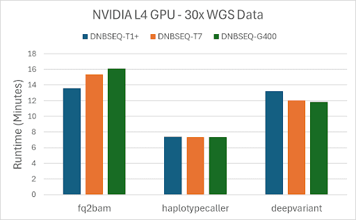
NVIDIA L4 GPU - 30x WGS DATA
DNBSEQ-T1+
DNBSEQ-T7
DNBSEQ-G400
|
Runtime
|
Cost
|
Runtime
|
Cost
|
Runtime
|
Cost
|
|
fq2bam
|
14
|
$1.51
|
15
|
$1.71
|
16
|
$1.79
|
|
haplotypecaller
|
7
|
$0.82
|
7
|
$0.82
|
7
|
$0.82
|
|
deepvariant
|
13
|
$1.47
|
12
|
$1.34
|
12
|
$1.32
|
As we expect, the runtime for the L40S instance is faster than the runtimes for the L4
instance, for each sample. This difference is reflected in the cost as well, shown in the
table below:
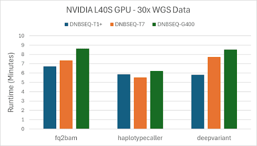
NVIDIA L40S GPU - 30x WGS DATA
DNBSEQ-T1+
DNBSEQ-T7
DNBSEQ-G400
|
Runtime
|
Cost
|
Runtime
|
Cost
|
Runtime
|
Cost
|
|
fq2bam
|
7
|
$1.68
|
7
|
$1.85
|
9
|
$2.17
|
|
haplotypecaller
|
6
|
$1.48
|
6
|
$1.39
|
6
|
$1.56
|
|
deepvariant
|
6
|
$1.46
|
8
|
$1.94
|
9
|
$2.14
|
## Concordance with the Truth Set
Aside from the runtime numbers, it’s important to check that the quality of the variants
matches closely with the truth set.
The NA12878 ground truth VCF can be found on the
[NIH FTP](https://ftp-trace.ncbi.nlm.nih.gov/ReferenceSamples/giab/release/NA12878_HG001/NISTv4.2.1/GRCh37/).
Since this VCF was run using the GRCh37 reference but our samples were run using UCSC
hg19 reference, we first need to do a liftover and then we can run concordance.
As an optional step, this can be done using the `liftover.sh` and
`concordance.sh` scripts respectively.
Below is a table of the results that we achieved using this workflow:
Table 6: Concordance results for the T7 sample from DeepVariant
|
Type
|
Filter
|
TRUTH.TP
|
TRUTH.FN
|
QUERY.FP
|
METRIC.Recall
|
METRIC.Precision
|
METRIC_F1_Score
|
|
INDEL
|
ALL
|
460832
|
6052
|
1389
|
0.987037
|
0.997107
|
0.992047
|
|
INDEL
|
PASS
|
460832
|
6052
|
1389
|
0.987037
|
0.997107
|
0.992047
|
|
SNP
|
ALL
|
3213043
|
38814
|
6106
|
0.988064
|
0.998104
|
0.993059
|
|
SNP
|
PASS
|
3213043
|
38814
|
6106
|
0.988064
|
0.998104
|
0.993059
|
Table 7: Concordance results for the T7 sample from HaplotypeCaller
|
Type
|
Filter
|
TRUTH.TP
|
TRUTH.FN
|
QUERY.FP
|
METRIC.Recall
|
METRIC.Precision
|
METRIC_F1_Score
|
|
INDEL
|
ALL
|
460832
|
6052
|
1389
|
0.987037
|
0.997107
|
0.992047
|
|
INDEL
|
PASS
|
460832
|
6052
|
1389
|
0.987037
|
0.997107
|
0.992047
|
|
SNP
|
ALL
|
3213043
|
38814
|
6106
|
0.988064
|
0.998104
|
0.993059
|
|
SNP
|
PASS
|
3213043
|
38814
|
6106
|
0.988064
|
0.998104
|
0.993059
|
Table 8: Concordance results for the G400 sample from DeepVariant
|
Type
|
Filter
|
TRUTH.TP
|
TRUTH.FN
|
QUERY.FP
|
METRIC.Recall
|
METRIC.Precision
|
METRIC_F1_Score
|
|
INDEL
|
ALL
|
459953
|
6931
|
2320
|
0.985155
|
0.995165
|
0.990135
|
|
INDEL
|
PASS
|
459953
|
6931
|
2320
|
0.985155
|
0.995165
|
0.990135
|
|
SNP
|
ALL
|
3208100
|
43757
|
7435
|
0.986544
|
0.997689
|
0.992085
|
|
SNP
|
PASS
|
3208100
|
43757
|
7435
|
0.986544
|
0.997689
|
0.992085
|
Table 9: Concordance results for the G400 sample from HaplotypeCaller
|
Type
|
Filter
|
TRUTH.TP
|
TRUTH.FN
|
QUERY.FP
|
METRIC.Recall
|
METRIC.Precision
|
METRIC_F1_Score
|
|
INDEL
|
ALL
|
459224
|
7660
|
5812
|
0.983593
|
0.987961
|
0.985772
|
|
INDEL
|
PASS
|
459224
|
7660
|
5812
|
0.983593
|
0.987961
|
0.985772
|
|
SNP
|
ALL
|
3199856
|
52001
|
47560
|
0.984009
|
0.985358
|
0.984683
|
|
SNP
|
PASS
|
3199856
|
52001
|
47560
|
0.984009
|
0.985358
|
0.984683
|
Just as we expect with Parabricks, we are seeing Precision and F1 scores upwards of 99%,
confirming that the variant callers are accurate with respect to the ground truth.
## Conclusion
In this guide, we showed how to download WGS data from Complete Genomics, run it through
alignment ([fq2bam](/tool-reference/tools/fq-2-bam-bwa-mem-gatk)) and variant calling ([haplotypecaller](/tool-reference/tools/haplotypecaller)
and [deepvariant](/tool-reference/tools/deepvariant)) on AWS, show the runtime and total cost per sample, and
finally demonstrated the concordance results against a truth set. Combined, this shows
that Parabricks supports data from Complete Genomics sequencers, in that it runs quickly
and accurately on the tools.