


Analytic Hessians in cuEST#
cuEST provides routines that help accelerate computationally demanding parts of analytic second derivatives (Hessians) of the energy with respect to nuclear coordinates. Analytic Hessians are used to compute harmonic vibrational frequencies and thermochemical corrections, to characterize stationary points as minima or transition states, and to provide accurate starting Hessians for geometry optimizations. Unlike finite differences of analytic gradients, analytic Hessians are free of step-size errors and numerical noise.
The Hessian routines evaluate derivatives of AO integrals and contract them with matrices that the caller supplies, so they are not tied to a particular electronic structure method. The same kinds of derivative integrals appear in the Hessians of many methods that use atom-centered basis functions, such as Hartree-Fock, Kohn-Sham DFT, MP2, and TDDFT. This guide uses the Hessian of a Hartree-Fock or Kohn-Sham DFT energy as an example of where the routines can be used.
Structure of the SCF Hessian#
This section applies only to self-consistent field (SCF) methods, that is, Hartree-Fock and Kohn-Sham DFT. The Hessians of other methods, such as MP2 and TDDFT, have additional contributions that are not described here.
For a converged SCF wavefunction, the Hessian with respect to the coordinates of atoms \(A\) and \(B\) can be written as the sum of two contributions.
Here, \(X_{A}\) denotes the Cartesian coordinates of atom \(A\), so each \(H_{AB}\) is a \(3 \times 3\) block.
The skeleton, \(H^{\rm skel}\), is the derivative of the analytic gradient with the density matrices held fixed. It consists of the second derivatives of the AO integrals, contracted with the unperturbed density matrices, together with the second derivative of the nuclear repulsion energy. Here and throughout this guide, the derivatives of the AO integrals include every way in which the integrals depend on the nuclear coordinates. Besides the motion of the atom-centered basis functions, this includes any other geometric dependence of the method, such as the motion of the integration grid points and the change in their partition weights, or the motion of the auxiliary basis functions and the response of the fit in density fitting. The skeleton collects all second-order geometric terms; the corresponding first-order terms enter the right-hand side described below.
The response term, \(H^{\rm resp}\), accounts for the relaxation of the molecular orbitals as the nuclei move. It requires the orbital response \(U^{A}\), the first-order change in the molecular orbital coefficients when atom \(A\) is displaced. The orbital response is the solution of the coupled-perturbed Hartree-Fock (CPHF) [1] [2] or Kohn-Sham (CPKS) [3] equations, a linear system \(L U^{A} = R^{A}\) with one right-hand side for each nuclear coordinate. The right-hand side, \(R^{A}\), is built from the first derivatives of the Fock matrix and overlap integrals with respect to \(X_{A}\), transformed to the MO basis. The left-hand side, \(L\), is the orbital Hessian, which contains no derivative integrals and is the same for every perturbation. \(H^{\rm resp}_{AB}\) is then assembled from the orbital response for one atom, the MO basis first-derivative matrices for the other, and Fock-like builds of the same kind as those used for the LHS.
The work of evaluating the Hessian therefore falls into three parts:
Skeleton: the second-derivative integrals, which give \(H^{\rm skel}\) directly.
Right-hand side (RHS): the Fock matrix nuclear derivatives, which define the CPHF/CPKS equations and enter \(H^{\rm resp}\).
Left-hand side (LHS): the orbital Hessian, which is applied to trial vectors to solve the CPHF/CPKS equations.
cuEST provides primitives to help accelerate parts of the skeleton and RHS through dedicated compute routines. For the LHS, the products of the orbital Hessian with trial vectors can be formulated in terms of Fock-like matrix contributions and evaluated with general cuEST API functions, such as those routinely used in ground-state energy calculations.
Note
Skeleton and RHS routines are currently available for the overlap (S) and kinetic energy (T) integrals. See Available Matrix Quantities for the status of each matrix quantity. Additional Hessian terms may appear in later cuEST releases.
Skeleton#
The skeleton follows from the analytic gradient of the SCF energy.
Here, \(D\) and \(W\) are the AO basis density and energy-weighted density matrices, and \(T\) and \(S\) are the kinetic energy and overlap matrices. The omitted terms are the corresponding contributions of the nuclear attraction, Coulomb, exchange, and exchange-correlation terms, including any grid or auxiliary basis terms, together with the derivative of the nuclear repulsion energy. The energy-weighted density matrix term has no counterpart in the energy. It arises because the molecular orbitals must remain orthonormal as the overlap of the basis functions changes with the nuclear positions.
The skeleton is the derivative of this gradient with respect to \(X_{B}\), with \(D\) and \(W\) held fixed.
The derivatives of \(D\) and \(W\) with respect to \(X_{B}\) give the response term, \(H^{\rm resp}\).
Both of the terms shown have the same form. Each contracts the second derivatives of an AO matrix \(O\) against a single AO basis matrix \(M\).
cuestKineticHessianSkeletonCompute() and cuestOverlapHessianSkeletonCompute() evaluate this
contraction for \(O = T\) and \(O = S\), with any AO basis matrix \(M\).
Right-Hand Side#
For a closed-shell Hartree-Fock reference in canonical orbitals, with \(i, j, k, l\) labeling occupied orbitals and \(a, b\) labeling virtual orbitals, the CPHF equations [4] read
where the right-hand side is
Here, \(\varepsilon_{i}\) are the orbital energies, \(S^{A}\) is the first derivative of the overlap matrix with respect to \(X_{A}\) in the MO basis, and \(F^{(A)}\) is the first derivative of the Fock matrix at fixed density. \(F^{(A)}\) is built from the derivatives of the kinetic energy, nuclear attraction, Coulomb, and exchange integrals, contracted with the unperturbed density and transformed to the MO basis. For Kohn-Sham DFT or density fitting, \(F^{(A)}\) also includes the corresponding first-order grid or auxiliary basis terms.
All of the derivative integrals in \(R^{A}\) enter through these MO basis first-derivative matrices. The RHS routines compute them one operator at a time.
cuestOverlapHessianRHSCompute() evaluates this transformation for \(O = S\), which gives
\(S^{A}\), and cuestKineticHessianRHSCompute() evaluates it for \(O = T\), which gives the
kinetic energy contribution to \(F^{(A)}\). The other contributions to \(F^{(A)}\) listed
above have the same form and are added to it. Several pairs of coefficient matrices can be
transformed in a single call (for example, the alpha and beta orbitals of an unrestricted
calculation).
Left-Hand Side#
The orbital Hessian, \(L\), contains no derivative integrals and is the same for every perturbation. Iterative solvers for the CPHF/CPKS equations never form \(L\) explicitly. Each product of \(L\) with a trial vector requires the Coulomb, exchange, and exchange-correlation contributions of a trial density, which can be built with the same routines as the SCF procedure (see Direct J and K, Density Fitting, and Grid-Based K).
Once \(U^{A}\) is known, \(H^{\rm resp}_{AB}\) is assembled from \(U^{B}\), the MO basis first-derivative matrices for atom \(A\), and further Fock-like builds of the type described above. No integral derivatives beyond those in the skeleton and RHS are required.
Blocking Perturbations#
The CPHF/CPKS equations for different perturbations share the orbital Hessian \(L\), but each has its own right-hand side and solution. The equations for different perturbations are therefore independent and can be solved one perturbation at a time or in blocks. The skeleton and RHS routines take explicit lists of atom indices, so that the derivative integrals can be blocked in the same way. Each atom in a list contributes three perturbations, one for each of its Cartesian coordinates, so a list of \(n\) atoms corresponds to \(3n\) perturbations. A call produces only the part of the result that belongs to the atoms in its lists. The Hessian can therefore be assembled from a sequence of calls over blocks of atoms, so that the GPU memory required at any one time is set by the size of a block rather than by the size of the molecule, as illustrated in Fig. 7.
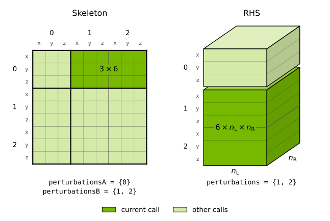
Fig. 7 Skeleton and RHS calls for a molecule with three atoms, divided into the blocks {0} and {1, 2}#
Each atom contributes three perturbations, one for each of its \(x\), \(y\), and
\(z\) coordinates. If \(A\) is the \(m\)-th atom in perturbationsA and
\(B\) is the \(m'\)-th atom in perturbationsB, element
\((3m+\alpha, 3m'+\beta)\) of the skeleton block is
where \(\alpha, \beta = 0, 1, 2\) label the \(x\), \(y\), and \(z\)
components. Similarly, if \(A\) is the \(m\)-th atom in perturbations, element
\((3m+\alpha, p, q)\) of the RHS tensor is
The highlighted skeleton call returns a \(3 \times 6\) block of 18 elements, and the highlighted RHS call returns a \(6 \times n_{\rm L} \times n_{\rm R}\) tensor.