Overview
This section describes the basic working principles of the cuTensorNet library. For a general introduction to quantum circuits, please refer to Introduction to quantum computing.
Introduction to tensor networks
Tensor networks emerge in many mathematical and scientific domains, ranging from quantum circuit simulation, quantum many-body physics, quantum chemistry, to machine learning. As network sizes scale up exponentially, there is an increasing need for a high-performance tensor network library in order to perform tensor network contractions efficiently, which cuTensorNet aims to serve.
Tensor and tensor network
Tensors are a generalization of scalars (0D), vectors (1D), and matrices (2D), to arbitrary number of dimensions. In the cuTensorNet library we follow cuTENSOR’s nomenclature:
A rank (or order) \(N\) tensor has \(N\) modes
Each mode has an extent (the size of the mode) and can be assigned a label (index) as part of the tensor network
Each mode has a stride accounting for the distance in physical memory between two logically consecutive elements along that mode, in unit of elements
For example, a \(3 \times 4\) matrix \(M\) has two modes (i.e., it’s a rank-2 tensor) of extent 3 and 4, respectively. In the C (row-major) memory layout, it has strides (4, 1). We can assign two mode labels, \(i\) and \(j\), to represent it as \(M_{ij}\).
Note
For NumPy/CuPy users, rank/order translates to the array attribute .ndim, the sequence of extents translates to .shape,
and the sequence of strides has the same meaning as .strides but in different units (NumPy/CuPy uses bytes instead of counts).
When two or more tensors are contracted to form another tensor, their shared mode labels are summed over. Diagrammatically, tensors and their contractions can be visualized as follows:
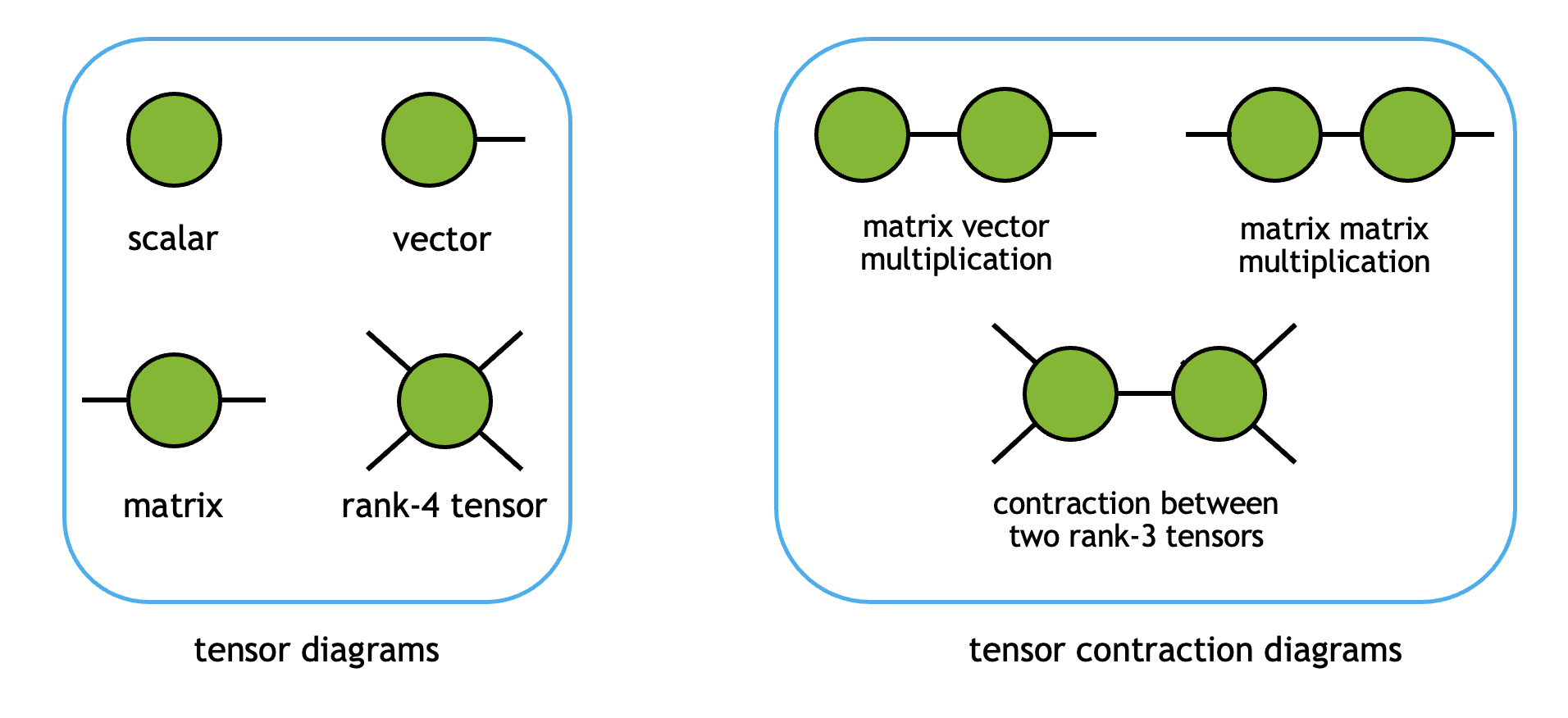
Here, each vertex represents one tensor object, and each edge stands for one mode label. When a mode label is contracted, the tensors are connected by the corresponding edges.
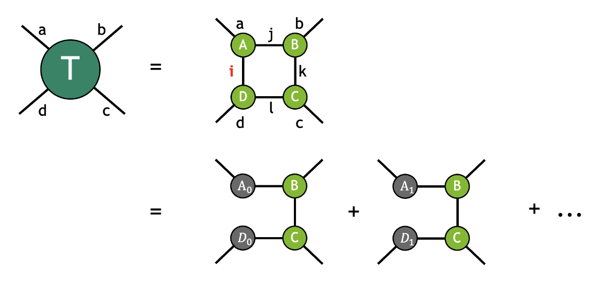
A tensor network is a collection of tensors contracted together to form an output tensor. The contractions between the constituent tensors fully determines the network topology. For example, the tensor \(T\) below is given by contracting the tensors \(A\), \(B\), \(C\), and \(D\):
where the modes with the same label are implicitly summed over following the Einstein summation convention. In this example, the mode label \(i\) connects the tensors \(D\) and \(A\), the mode label \(j\) connects the tensors \(A\) and \(B\), the mode label \(k\) connects the tensors \(B\) and \(C\), the mode label \(l\) connects the tensors \(C\) and \(D\). The four uncontracted modes with labels \(a\), \(b\), \(c\), and \(d\) refer to free modes (sometimes also referred to as external modes), indicating the resulting tensor \(T\) is of rank 4. Following the diagrammatic convention above, this contraction can be visualized as follows:
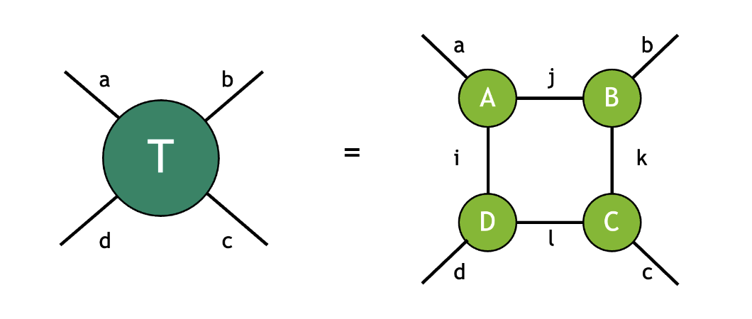
As we can see from the diagram, this contraction has a square topology where each tensor is connected to its adjacent tensors.
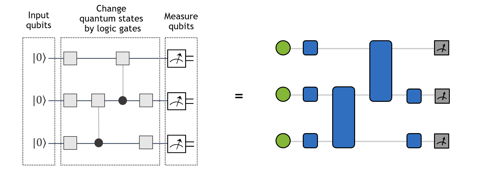
Similarly, quantum circuits can be viewed as a kind of tensor networks. As shown in the figure below, single-qubit and two-qubit gates translate to rank-2 and rank-4 tensors, respectively. Meanwhile, the initial single-qubit states \(|0\rangle\) and single-qubit measurement operations can be viewed as vectors (projectors) of size 2. The contraction of the tensor network on the right yields the wavefunction amplitude of the left circuit for a particular basis state (ex: \(|010\rangle\)).
Description of tensor networks
A full description of a given tensor network contraction requires two pieces of information: tensor operands and topology of the network.
A tensor network in the cuTensorNet library is represented by the
cutensornetNetworkDescriptor_t descriptor that effectively encodes the topology and data
type of the network. To be precise, this descriptor specifies the number of input tensors in numInputs
and the number of modes for each tensor in the array numModesIn, along with each tensor’s modes, extents, and
strides in the arrays of pointers modesIn, extentsIn, and stridesIn, respectively.
The tensor network descriptor also accepts an array of qualifiers (qualifiersIn) which correspond to each input tensor,
in which, each input tensor can be flagged as Conjugate (default non-Conjugate).
When an input tensor is flagged Conjugate, its data will be conjugated upon contraction.
Likewise, it holds similar information about the output tensor (e.g., numModesOut, modesOut, extentsOut, stridesOut).
Note that there is only one output tensor per network, so there is no need to set numOutputs and
the corresponding arguments are just plain arrays.
It is possible for all these network metadata to live on the host, since when constructing a tensor network only its topology and the data-access pattern matter; we do not need to know the actual content of the input tensors at network descriptor creation.
Internally, cuTensorNet utilizes cuTENSOR to create tensor objects and perform pairwise tensor contractions.
cuTensorNet’s APIs are designed such that users can just focus on creating the network description without having to manage such
“low-level” details themselves.
The tensor contraction can be computed in a different precision from the data type, given by a cutensornetComputeType_t constant.
Once a valid tensor network is created, one can
Find a low-cost contraction path, possibly with slicing and additional constraints
Access information concerning the contraction path
Get the needed workspace size to accommodate intermediate tensors
Create a contraction plan according to the info collected above
Auto tune the contraction plan to optimize the runtime of the network contraction
Perform the actual contraction to retrieve the output tensor
It is the users’ responsibility to manage device memory for the workspace (from Step 3) and input/output tensors (for Step 5). See API Reference for the cuTensorNet APIs (section Workspace Management API). Alternatively, the user can provide a stream-ordered memory pool to the library to facilitate workspace memory allocations, see Memory Management API for details.
Approximate tensor network algorithms
While contraction path optimization can greatly reduce the computational cost for exact contraction of a network, the cost can still quickly scale beyond classical computers limit as the network size and complexity increases. A variety of approximate tensor network methods have been developed to address this challenge, like algorithms based on matrix product states (MPS). These methods often aim to exploit the sparsity in the network using tensor decomposition techniques such as QR and SVD.
The QR and SVD decompositions of a tensor can be visualized by the diagram below and can be viewed as the higher order generalization of matrix QR/SVD.
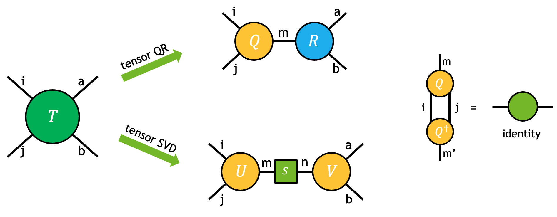
The problem can be fully specified by user-requested partitions of modes in the output tensors. For example, the tensor \(T\) in the figure above is decomposed into output tensors \(U\), \(S\), and \(V\) using tensor SVD:
Note
Although the output \(S\) is represented as a matrix in the equation and the diagram, only its diagonal elements are nonzero. In all SVD-related APIs of cuTensorNet, only the non-zero diagonal elements are returned (as a vector).
Once the partition of modes in \(U\) and \(V\) is determined, input tensor \(T\) is first permuted to an intermediate tensor \(\bar{T}\) with the proper mode ordering such that it can be viewed as a matrix for the decomposition:
After the matrix SVD/QR decomposition, permutation may still be needed to transform the output intermediate tensors \(\bar{U}\) and \(\bar{V}\), to the requested output \(U\) and \(V\).
Note
Tensor SVD and QR in cuTensorNet operate in reduced mode, i.e., \(k=min(m, n)\) where k denotes the extent of the shared mode of the output, while m and n represent the effective input matrix row/column sizes. While tensor QR is always exact, cuTensorNet provides different ways for users to truncate singular values, \(\bar{U}\), and \(\bar{V}\). For instance, if the user wishes to perform fixed extent truncation in tensor SVD, \(k\) can be set to be lower than \(min(m, n)\). See SVD options for detailed descriptions.
In practice, tensor decomposition and pairwise tensor contraction are often combined to transform the original network to a new topology that reflects its internal sparsity or entanglement geometry in the field of quantum simulation. For instance, in matrix product states (MPS) simulator, the qubits states are mapped to a 1-dimensional tensor chain. When gate tensors are applied to the MPS, a sequence of contraction and tensor QR/SVD operations are performed to ensure that the output states are still represented as a 1-dimensional tensor chain. The compound operation that is used to maintain the MPS geometry is termed as the gate split process. For example, a two-qubit gate tensor \(G\) is applied to two connecting tensors \(A\) and \(B\) to generate output tensors \(\tilde{A}\) and \(\tilde{B}\) with similar modes as \(A\) and \(B\):
In the gate split process, the number of singular values may also be truncated to keep the MPS size tractable. By iterating this process throughout the network, the original tensor network can be approximated by the output MPS states. The process can be diagrammatically shown as below:
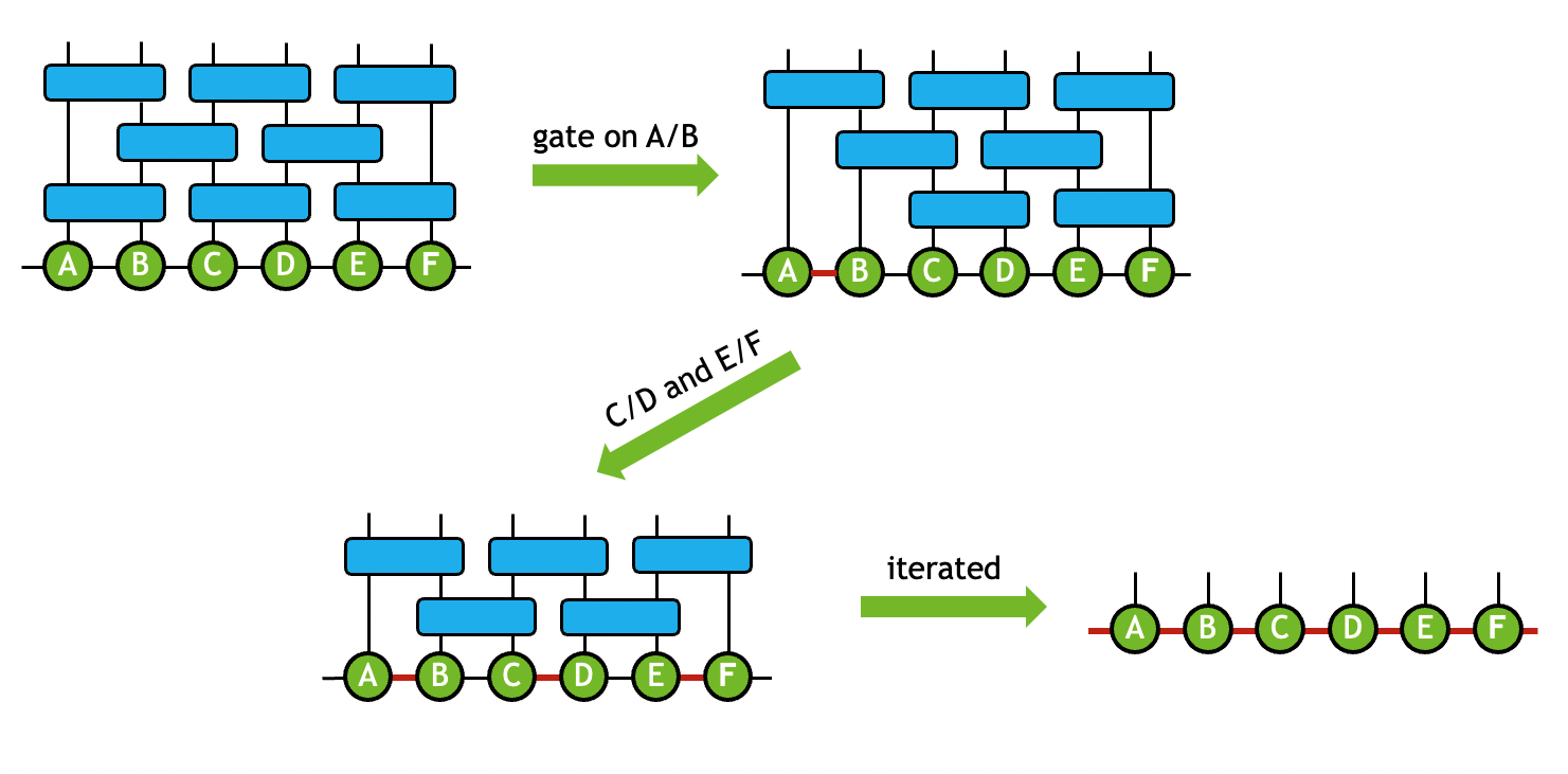
For more detailed explanation of how the transformation is performed, please refer to Gate Split Algorithm below.
Contraction Optimizer
A contraction path is a sequence of pairwise contractions represented in the numpy.einsum_path() format.
For a given tensor network, the contraction cost can differ by orders of magnitude, depending on the quality of the contraction path.
Therefore, it is crucial to use a path optimizer to find a contraction path that minimizes the total cost of contracting the tensor network.
Currently, the contraction cost refers to the floating point operations (FLOP) for the cuTensorNet path optimizer’s purpose, and an optimal
contraction path corresponds to the path with the minimal FLOP count.
The cuTensorNet path optimizer is based on a graph-partitioning approach (called phase 1), followed by interleaved slicing and reconfiguration optimization (called phase 2).
Practically, experience indicates that finding an optimal contraction path can be sensitive to the choice of configuration parameters,
which can be configured via cutensornetContractionOptimizerConfigSetAttribute() and queried via cutensornetContractionOptimizerConfigGetAttribute(). The rest of this section aims to introduce the overall optimization scheme and these configurable parameters.
Once the optimization completes, it returns an opaque object cutensornetContractionOptimizerInfo_t that contains all of the attributes for creating a contraction plan. For example, the optimal path (CUTENSORNET_CONTRACTION_OPTIMIZER_INFO_PATH) and the corresponding FLOP count (CUTENSORNET_CONTRACTION_OPTIMIZER_INFO_FLOP_COUNT) can be queried via cutensornetContractionOptimizerInfoGetAttribute().
Note
The returned FLOP count assumes the input tensors are real-valued; for complex-valued tensors, multiplying it by 4 is a good estimation.
Alternatively, we can bypass the cuTensorNet optimizer entirely by supplying your own path using cutensornetContractionOptimizerInfoSetAttribute(). For the unset cutensornetContractionOptimizerInfo_t attributes (ex: the number of slices and the FLOP) cuTensorNet will either use the default values or compute them on the fly when applicable.
Graph partitioning
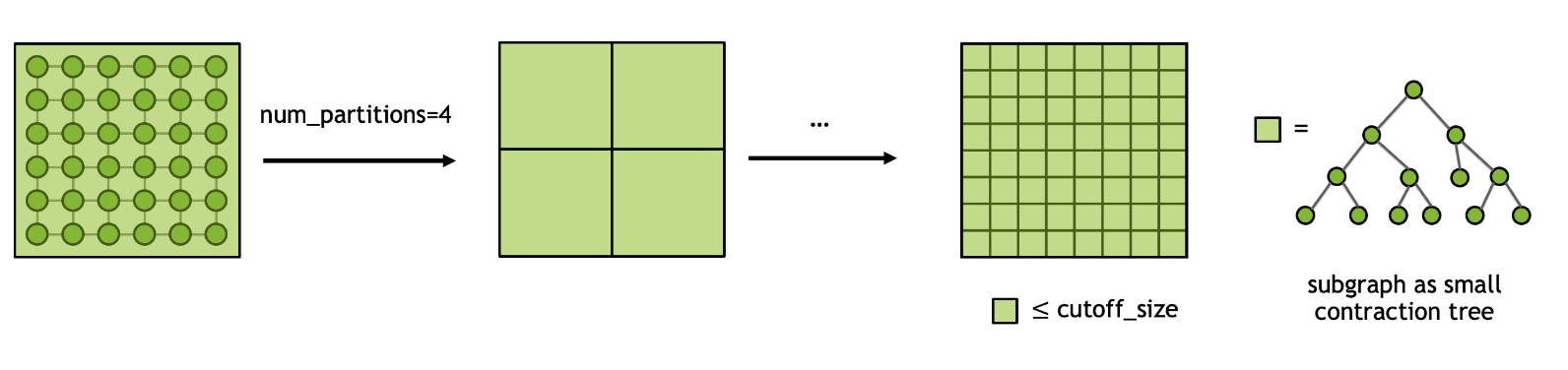
In general, searching for the optimal contraction path for a given tensor network is a NP-hard problem. Therefore, it is crucial to approach this problem in a divide-and-conquer spirit. Given an input tensor network, we first perform graph partitioning to split the network into N smaller subgraphs and repeat this process recursively until the size of each subgraph is less than the cutoff size. Once the final partitioning scheme is determined, finding the paths for contracting first within each subgraph and then all subgraphs becomes tractable. The process can be illustrated using the diagram below and we get a coarse contraction path or contraction tree for subsequent optimizations.
The cuTensorNet library provides controls over the graph partition algorithms through following parameters:
CUTENSORNET_CONTRACTION_OPTIMIZER_CONFIG_GRAPH_NUM_PARTITIONS: The number of subgraphs to partition into within each loop.
CUTENSORNET_CONTRACTION_OPTIMIZER_CONFIG_GRAPH_CUTOFF_SIZE: The maximal size allowed for each subgraph until the partitioning is completed.
CUTENSORNET_CONTRACTION_OPTIMIZER_CONFIG_GRAPH_ALGORITHM: The graph algorithm to be used in graph partitioning. Default is set to CUTENSORNET_GRAPH_ALGO_KWAY.
CUTENSORNET_CONTRACTION_OPTIMIZER_CONFIG_GRAPH_IMBALANCE_FACTOR: The maximum allowed size imbalance among the partitions.
CUTENSORNET_CONTRACTION_OPTIMIZER_CONFIG_GRAPH_NUM_ITERATIONS: The number of iterations for the refinement algorithms at each stage of the uncoarsening process of the graph partitioner.
CUTENSORNET_CONTRACTION_OPTIMIZER_CONFIG_GRAPH_NUM_CUTS: The number of different partitionings that the graph partitioner will compute.
Slicing
In order to fit a tensor network contraction into available device memory, as specified by workspaceSizeConstraint, it may be necessary to use slicing (also known as variable projection or bond cutting).
By slicing, we split the contraction of the entire tensor network into a number of independent smaller contractions where each contraction considers only one particular position
of a certain mode (or combination of modes). The total number of slices that are created equals the product of the extents of the sliced modes.
The result for full tensor network contraction can be obtained by summing over the output of each sliced contraction.
Taking the above \(T\) tensor as an example, if we slice over the mode i we obtain the following representation:
As one can see from the diagram, the sliced mode \(i_s\) is no longer implicitly summed over as part of tensor contraction, but instead explicitly summed in the last step. As a result, slicing can effectively reduce the memory footprint for contracting large tensor networks, in particular quantum circuits. Besides, since each sliced contraction is independent from the others, the computation can be efficiently parallelized in various distributed settings.
Despite all the benefits above, the downside of slicing is that it often increases the total FLOP count of the entire contraction. The overhead of slicing heavily depends on the contraction path and the modes that are sliced. In general, there is no simple way to determine the best set of modes to slice.
The slice-finding algorithm in the cuTensorNet library can be tuned by following parameters:
CUTENSORNET_CONTRACTION_OPTIMIZER_CONFIG_SLICER_DISABLE_SLICING: If set to 1, slicing will not be considered, regardless of available memory. Default is 0.
CUTENSORNET_CONTRACTION_OPTIMIZER_CONFIG_SLICER_MEMORY_MODEL: Specifies the memory model used to determine the workspace size, seecutensornetMemoryModel_t. The default is to use a memory model compatible with cuTENSOR (CUTENSORNET_MEMORY_MODEL_HEURISTIC).
CUTENSORNET_CONTRACTION_OPTIMIZER_CONFIG_SLICER_MEMORY_FACTOR: The memory limit for the first slice-finding iteration as a percentage of the workspace size. The default is 80 when usingCUTENSORNET_MEMORY_MODEL_CUTENSORfor the memory model and 100 when usingCUTENSORNET_MEMORY_MODEL_HEURISTIC.
CUTENSORNET_CONTRACTION_OPTIMIZER_CONFIG_SLICER_MIN_SLICES: Specifies the minimum number of slices to produce (e.g. to create parallelizable work). Default is 1.
CUTENSORNET_CONTRACTION_OPTIMIZER_CONFIG_SLICER_SLICE_FACTOR: Specifies the factor by which the number of slices will increase per slice-finding iteration. For example, if the previous iteration had \(N\) slices and the slice factor is \(s\), the next iteration will produce at least \(sN\) slices. Since reconfiguration (see below) occurs after each slice-finding iteration, increasing this value will decrease the amount of reconfiguration, which, in turn, will decrease the amount of time taken but probably worsen the quality of the contraction tree. Default is 32. Must be at least 2. A small value of this factor (for example 2 or 4) is recommended when the number of slices requested or required is very large, because it provide a better quality of slices.
The slice-finding algorithm in the cuTensorNet library utilizes a set of heuristics and the process can be coupled with the subtree reconfiguration routine to
find the optimal set of modes that both satisfies the memory constraint and incurs the least overhead.
Reconfiguration
At the end of each slice-finding iteration, the quality of the contraction tree has been diminished by the slicing. We can improve the contraction tree at this stage by performing reconfiguration. Reconfiguration considers a number of small subtrees within the full contraction tree and attempts to improve their quality. The repeated process of slicing and reconfiguration can be viewed as illustrated in the diagram below.

Although this process is computationally expensive, a sliced contraction tree without reconfiguration may be orders of magnitude more expensive to execute than expected. The cuTensorNet library offers some controls to influence the reconfiguration algorithm:
CUTENSORNET_CONTRACTION_OPTIMIZER_CONFIG_RECONFIG_NUM_ITERATIONS: Specifies the number of subtrees to consider during each reconfiguration. The amount of time spent in reconfiguration, which usually dominates the optimizer run time, is linearly proportional to this value. Based on our experiments, values between 500 and 1000 provide very good results. Default is 500. Setting this to 0 will disable reconfiguration.
CUTENSORNET_CONTRACTION_OPTIMIZER_CONFIG_RECONFIG_NUM_LEAVES: Specifies the maximum number of leaf nodes in each subtree considered by reconfiguration. Since the time spent is exponential in this quantity for optimal subtree reconfiguration, selecting large values will invoke faster non-optimal algorithms. Nonetheless, the time spent by reconfiguration increases very rapidly as this quantity is increased. Default is 8. Must be at least 2. While using the default value usually produces the best FLOP count, setting it to 6 will speed up the optimizer execution without significant increase in the FLOP count for many problems.
Deferred rank simplification
Since the time taken by the path-finding algorithm increases quickly as the number of tensors increases, it is advantageous to minimize the number of tensors, if possible. Rank simplification removes trivial tensor contractions from the network in order to improve performance. These contractions are those where a tensor is only connected with at most two neighbors, effectively making the contraction a small matrix-vector or matrix-matrix multiplication. One example for rank simplification is given in the figure below:
This technique is particularly useful for tensor networks with low connectivity; for instance, all single-qubit gates in quantum circuits can be fused with the neighboring multi-qubit gates, thereby reducing the search space for the optimizer. The necessary contractions to perform the simplification are not immediately performed, but, rather, are prepended to the contraction path returned. If, for some reason, such simplification is not desired, it can be disabled:
CUTENSORNET_CONTRACTION_OPTIMIZER_CONFIG_SIMPLIFICATION_DISABLE_DR: If set to 1, simplification will be skipped. This will run the path-finding algorithm on the full tensor network, increasing the time needed. Default is 0.
While simplification helps lower the FLOP count in most cases, it may sometimes (depending on the network topology and other factors) lead to a path with a higher FLOP count. We recommend that users experiment with the impact of turning simplification off (using the option listed above) on the computed path.
Hyper-optimizer
cuTensorNet provides a hyper-optimizer for the path optimization that can automatically generate
many instances of contraction paths and return the best of them in terms of the total FLOP count.
The number of instances is user-controlled via the use of CUTENSORNET_CONTRACTION_OPTIMIZER_CONFIG_HYPER_NUM_SAMPLES which is set to 0 by default.
The idea here is that the hyper-optimizer will create
CUTENSORNET_CONTRACTION_OPTIMIZER_CONFIG_HYPER_NUM_SAMPLES instances, each reflecting the use of different parameters within the optimizer algorithm.
Each instance will run the full optimizer algorithm including reconfiguration and slicing (if requested).
At the end of the hyper-optimizer loop, the best path (in term of FLOP counts) is returned.
The hyper-optimizer runs its instances in parallel.
The desired number of threads can be set using CUTENSORNET_CONTRACTION_OPTIMIZER_CONFIG_HYPER_NUM_THREADS
and is chosen to be half of the available logical cores by default. The number of threads
is limited to the number of the available logical cores to avoid the resource contention that is likely with a larger number of threads.
Internally, cuTensorNet holds a thread pool for multithreading in the hyper-optimizer etc. The thread pool lifetime is bound to the cuTensorNet handle. (In previous releases, OpenMP was used; this is no longer the case since cuTensorNet v2.0.0.)
The configuration parameters that are varied by the hyper-optimizer can be found in the graph partitioning section.
Some of these parameters may be fixed to a given value (via cutensornetContractionOptimizerConfigSetAttribute()). When a parameter is fixed, the hyper-optimizer will not randomize it. The randomness can be fixed by setting the seed via the attribute CUTENSORNET_CONTRACTION_OPTIMIZER_CONFIG_SEED.
Approximation setting
SVD Options
In addition to the standard tensor SVD mentioned above, cuTensorNet allows users to perform truncation, normalization, and re-partition
during the decomposition. For truncation, the most common strategy is to keep the largest k number of singular values and trim out the remaining ones.
In cuTensorNet, this can be easily specified by modifying the extent of the shared mode in the output cutensornetTensorDescriptor_t object.
Alternatively, users may truncate the singular values based on the actual value or the distribution of the eigenvalues during runtime.
Such truncation setting, along with normalization and re-partition options are provided by different attributes of the cutensornetTensorSVDConfig_t object:
CUTENSORNET_TENSOR_SVD_CONFIG_ABS_CUTOFF: The cutoff for the largest singular value during truncation. Eigenvalues that are smaller will be trimmed out.
CUTENSORNET_TENSOR_SVD_CONFIG_REL_CUTOFF: The cutoff for the maximal singular value relative to the largest eigenvalue. Eigenvalues that are smaller than this fraction of the largest singular value will be trimmed out.
CUTENSORNET_TENSOR_SVD_S_NORMALIZATION: Whether to normalize certain norm of the truncated singular values to 1. Default is no.
CUTENSORNET_TENSOR_SVD_S_PARTITION: Whether to partition the singular values onto u, or v, or both u and v. Default is no.
Note
The value-based truncation options in cutensornetTensorSVDConfig_t can be used in conjuction with the fixed extent truncation, but since the actual reduced extent found at runtime is unknown,
the size of the data allocation for the output tensors should always be based on the assumption of no value-based truncation. After the execution, the potentially reduced extent found at runtime will
be stored in the CUTENSORNET_TENSOR_SVD_INFO_REDUCED_EXTENT attribute of cutensornetTensorSVDInfo_t and also reflected in the output cutensornetTensorDescriptor_t.
Users can either call cutensornetTensorSVDInfoGetAttribute() or cutensornetGetTensorDetails() to query this information.
Gate split algorithm
In general there are more than one approache to perform the gate split operation.
cuTensorNet provides two algorithms in cutensornetGateSplitAlgo_t for this purpose:
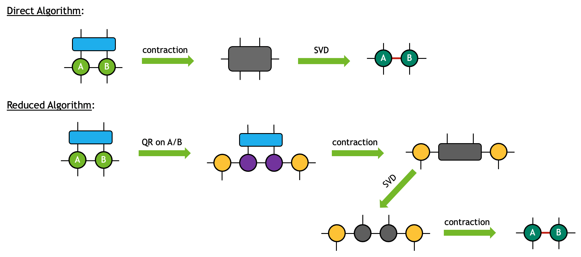
CUTENSORNET_GATE_SPLIT_ALGO_DIRECT: The three input tensors will first be contracted to form an intermediate tensor. A subsequent tensor SVD will take place to decompose the intermediate tensor to the desired output. This algorithm is generally more memory demanding but more performant when the tensor sizes are relatively small.
CUTENSORNET_GATE_SPLIT_ALGO_REDUCED: The input tensors A and B will first be decomposed into smaller fragments via tensor QR. The twoRtensors from the decomposition will then be contracted with input tensorGto form an intermediate tensor. A subsequent tensor SVD will take place to decompose the intermediate tensor, the output of which will then contract with theQtensors from the first step to form the desired outputs. This algorithm is generally less memory demanding and more performant when the tensors sizes get large.
Note
For CUTENSORNET_GATE_SPLIT_ALGO_REDUCED, cuTensorNet may internally skip QR on tensor A or/and B if no memory size reduction
can be achieved in the decomposition.
The two algorithms can be diagrammatically visualized as follows (singular values are partitioned equally onto the two outputs in this example):
Supported data types
For tensor nework contraction, a valid combination of the data and compute types inherits in a straightforward fashion from
that of cuTENSOR. Please refer to cutensornetCreateNetworkDescriptor() and cuTENSOR’s User Guide for details.
For approximate tensor network functionalities including tensor SVD/QR decompositions and gate split operation, following data types are supported:
Note
For gate split operation, the valid compute types for the data types above are consistent with that of tensor network contraction.
References
For a technical introduction to cuTensorNet, please refer to the NVIDIA blog:
For further information about general tensor networks, please refer to the following:
For the application of tensor networks to quantum circuit simulations, please see:
For citing cuQuantum, please see:
“NVIDIA/cuQuantum: cuQuantum v22.11”, NVIDIA cuQuantum team, 2022, DOI:10.5281/zenodo.6385574.