> For clean Markdown of any page, append .md to the page URL.
> For a complete documentation index, see https://docs.nvidia.com/cuvs/llms.txt.
> For full documentation content, see https://docs.nvidia.com/cuvs/llms-full.txt.
> For AI client integration (Claude Code, Cursor, etc.), connect to the MCP server at https://docs.nvidia.com/cuvs/_mcp/server.
# What is Vector Search?
## Introduction
Vector search finds the vectors that are closest to a query vector. Those nearest-neighbor results are the backbone of semantic search, retrieval-augmented generation, recommender systems, duplicate detection, clustering workflows, and many other vector data applications.
The simplest way to find nearest neighbors is exact search: compare the query with every vector, compute every distance, and return the closest results. This gives the true nearest neighbors, but it becomes expensive as datasets grow because every query has to do more distance work.
Approximate nearest-neighbor (ANN) indexes make that work cheaper. They usually do this in one or both of two ways: make each vector comparison cheaper, or reduce the number of vector comparisons that need to be computed. These trade exactness for speed, memory efficiency, or scale.
In vector search, [recall](/cuvs/user-guide/benchmarking-guide/methodologies#recall) is the main quality metric. It measures how many of the exact nearest neighbors were returned by the approximate search. Higher recall usually costs more build time, more search time, more memory, or some combination of all three.
This page introduces the main techniques used to reduce vector search cost, then explains how those techniques scale into larger index and database architectures. By the end, you should have a practical starting point for choosing an index type and understanding the key attributes, benefits, and tradeoffs of each option.
## Reducing the Footprint
Reducing the footprint means making each vector cheaper to store, move, or compare. This can reduce memory use, improve cache behavior, and lower memory bandwidth pressure during search. The main tradeoff is that smaller representations are often less precise, so they may need refinement or more careful tuning. For a broader overview of vector compression methods, see [Compression](/cuvs/getting-started/introduction/compression).
### Quantization
Quantization compresses vectors so they use less memory and require less bandwidth during search. It can be used with many index types, not just inverted file (IVF) indexes. The main tradeoff is that compression usually improves speed and memory efficiency at the cost of some recall.
Graph-based indexes can often be built directly over quantized vectors. In that case, the compressed representation is part of graph construction and search.
IVF indexes usually apply quantization inside the partitioned structure. Because IVF first divides the dataset into coarse partitions, each partition can be compressed locally. This can improve the quality of the compressed representation while still reducing memory traffic during search.
### Dimensionality Reduction
Dimensionality reduction makes vectors shorter by projecting them into fewer dimensions. Shorter vectors require fewer operations per distance calculation and less memory per vector. This is useful when the original vectors contain redundant or noisy dimensions, or when the search system is limited by memory bandwidth.
[PCA](/cuvs/user-guide/api-guides/preprocessing-guide/pca) is a common linear method that preserves the directions with the most variance. [Spectral Embedding](/cuvs/user-guide/api-guides/preprocessing-guide/spectral-embedding) is graph-based and can preserve local neighborhood structure when the data lies on a lower-dimensional manifold. These methods can reduce search cost, but they add preprocessing work and may remove information that matters for nearest-neighbor quality.
Dimensionality reduction can also be combined with quantization. A workflow might first project vectors into a smaller space, then quantize the result to reduce memory bandwidth even further.
### Refinement / Reranking
Refinement, often called reranking, is a way to recover accuracy after an approximate or compressed search. The index first uses a fast representation, such as quantized or lower-dimensional vectors, to find a candidate set. Then it recomputes distances for those candidates using a more accurate representation, often the original full-precision vectors.
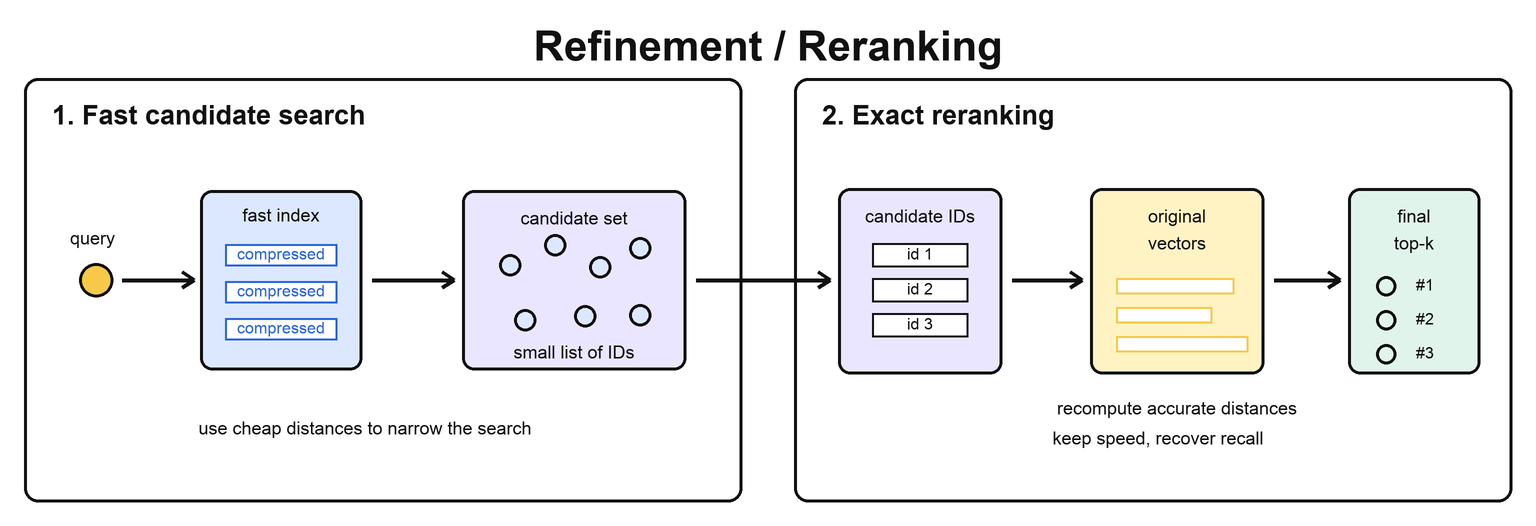 This is especially useful with quantized indexes. Quantization makes search faster and smaller, but compressed distances are approximate. Reranking lets the system use compressed vectors to quickly narrow the search, then use full-precision vectors to choose the final nearest neighbors.
For example, an [IVF-SQ](/user-guide/api-guides/indexing-guide/ivf-flat#ivf-sq-and-scalar-quantization) or [IVF-PQ](/user-guide/api-guides/indexing-guide/ivf-pq) index may use compressed vectors to scan selected partitions quickly. After it finds the best candidate IDs, a refinement step can load the original vectors for those candidates and compute exact distances. This usually improves recall while keeping most of the speed and memory benefits of compressed search.
[ScaNN](/user-guide/api-guides/indexing-guide/sca-nn) also relies heavily on this idea: it prunes the dataset quickly using partitioning and quantization, then reranks a smaller candidate set to improve final result quality.
## Reducing Distances
The other major strategy is to avoid comparing the query against most of the dataset. These indexes build a structure that guides each query toward promising candidates, then compute distances only for those candidates.
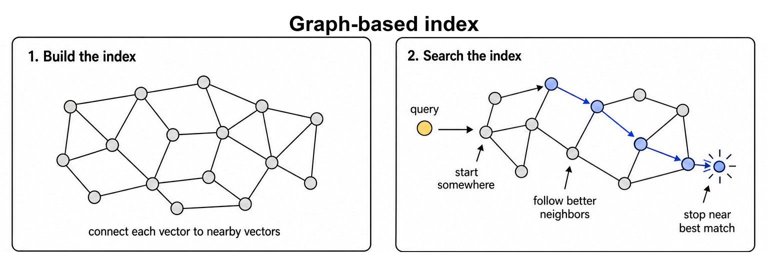
### Graph-based Algorithms
Graph-based indexes connect nearby vectors into a navigation structure. A query moves through the graph toward better candidates rather than scanning every vector. [HNSW](/user-guide/api-guides/indexing-guide/cagra#interoperability-with-hnsw) is a strong CPU graph index, [CAGRA](/user-guide/api-guides/indexing-guide/cagra) is optimized for GPU graph search and fast GPU graph construction, and [Vamana/DiskANN](/user-guide/api-guides/indexing-guide/vamana) is designed for very large or disk-backed graph search.
This is especially useful with quantized indexes. Quantization makes search faster and smaller, but compressed distances are approximate. Reranking lets the system use compressed vectors to quickly narrow the search, then use full-precision vectors to choose the final nearest neighbors.
For example, an [IVF-SQ](/user-guide/api-guides/indexing-guide/ivf-flat#ivf-sq-and-scalar-quantization) or [IVF-PQ](/user-guide/api-guides/indexing-guide/ivf-pq) index may use compressed vectors to scan selected partitions quickly. After it finds the best candidate IDs, a refinement step can load the original vectors for those candidates and compute exact distances. This usually improves recall while keeping most of the speed and memory benefits of compressed search.
[ScaNN](/user-guide/api-guides/indexing-guide/sca-nn) also relies heavily on this idea: it prunes the dataset quickly using partitioning and quantization, then reranks a smaller candidate set to improve final result quality.
## Reducing Distances
The other major strategy is to avoid comparing the query against most of the dataset. These indexes build a structure that guides each query toward promising candidates, then compute distances only for those candidates.
### Graph-based Algorithms
Graph-based indexes connect nearby vectors into a navigation structure. A query moves through the graph toward better candidates rather than scanning every vector. [HNSW](/user-guide/api-guides/indexing-guide/cagra#interoperability-with-hnsw) is a strong CPU graph index, [CAGRA](/user-guide/api-guides/indexing-guide/cagra) is optimized for GPU graph search and fast GPU graph construction, and [Vamana/DiskANN](/user-guide/api-guides/indexing-guide/vamana) is designed for very large or disk-backed graph search.
 Graph indexes often provide strong recall and latency tradeoffs because search follows local neighbor relationships. The cost is that graph construction can be more expensive than simpler partitioned indexes, and the graph links add memory overhead.
### Locality-sensitive Hashing
Locality-sensitive hashing (LSH) uses hash functions that are designed to place similar vectors into the same buckets with high probability. During search, the query is hashed, then the system compares against vectors in matching or nearby buckets instead of scanning the full dataset.
This is different from ordinary hash partitioning. Ordinary hashing is useful for distributing data, but it does not preserve vector similarity. LSH tries to preserve similarity in the hash assignment itself. In practice, LSH often needs multiple hash tables, larger candidate sets, or extra probing to reach high recall, so modern vector search systems more often rely on graph-based or tree-style indexes. It is still an important concept because it shows the same core idea: use structure to avoid unnecessary distance calculations.
### Tree-based
Tree-based algorithms reduce distance work by routing a query through a hierarchy of partitions. Classic examples include kd-trees, ball trees, vantage-point trees, and random projection trees. These methods work best when the routing structure can quickly rule out large parts of the dataset, though many classic tree methods become less effective as vector dimensionality grows.
In vector search, inverted file (IVF) indexes are often treated as a tree-style architecture. An IVF index is a shallow tree: the coarse routing layer contains centroids, and the leaves are inverted lists that store vectors assigned to those centroids. During build, the index trains coarse centroids, often with k-means, and assigns each vector to the closest centroid. During search, the query first chooses a small number of nearby centroids, then scans only the vectors in those lists.
Graph indexes often provide strong recall and latency tradeoffs because search follows local neighbor relationships. The cost is that graph construction can be more expensive than simpler partitioned indexes, and the graph links add memory overhead.
### Locality-sensitive Hashing
Locality-sensitive hashing (LSH) uses hash functions that are designed to place similar vectors into the same buckets with high probability. During search, the query is hashed, then the system compares against vectors in matching or nearby buckets instead of scanning the full dataset.
This is different from ordinary hash partitioning. Ordinary hashing is useful for distributing data, but it does not preserve vector similarity. LSH tries to preserve similarity in the hash assignment itself. In practice, LSH often needs multiple hash tables, larger candidate sets, or extra probing to reach high recall, so modern vector search systems more often rely on graph-based or tree-style indexes. It is still an important concept because it shows the same core idea: use structure to avoid unnecessary distance calculations.
### Tree-based
Tree-based algorithms reduce distance work by routing a query through a hierarchy of partitions. Classic examples include kd-trees, ball trees, vantage-point trees, and random projection trees. These methods work best when the routing structure can quickly rule out large parts of the dataset, though many classic tree methods become less effective as vector dimensionality grows.
In vector search, inverted file (IVF) indexes are often treated as a tree-style architecture. An IVF index is a shallow tree: the coarse routing layer contains centroids, and the leaves are inverted lists that store vectors assigned to those centroids. During build, the index trains coarse centroids, often with k-means, and assigns each vector to the closest centroid. During search, the query first chooses a small number of nearby centroids, then scans only the vectors in those lists.
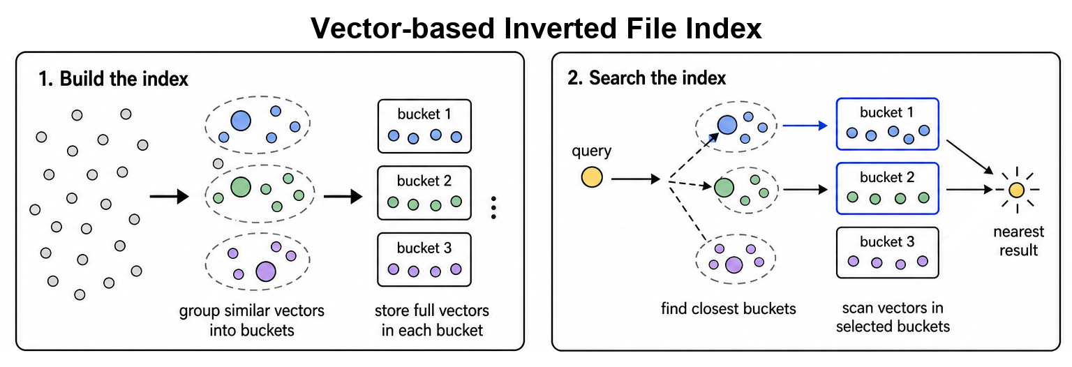 IVF indexes are useful because search cost depends on how many lists are probed, not directly on the full dataset size. [IVF-Flat](/user-guide/api-guides/indexing-guide/ivf-flat) stores full-precision vectors inside each list, [IVF-SQ](/user-guide/api-guides/indexing-guide/ivf-flat#ivf-sq-and-scalar-quantization) adds scalar quantization to reduce memory bandwidth, and [IVF-PQ](/user-guide/api-guides/indexing-guide/ivf-pq) uses product quantization for stronger compression.
## Scaling Vector Indexes
At larger scale, the index design becomes part of the storage and serving architecture. Systems may partition data for operations, partition data by semantic locality, move colder data to disk, or use GPUs to accelerate expensive stages of preprocessing, clustering, index build, and search.
### Hash Partitioning
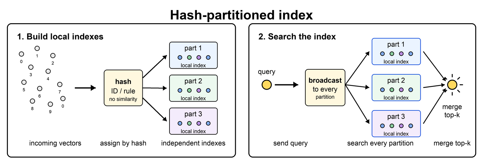
Any ANN index can be scaled out in a simple way by splitting vectors into multiple independent partitions, then building a separate index for each partition. The partitions might be assigned by hashing an ID, by ingestion segment, or by another rule that does not use vector similarity.
This is easy to operate because each partition can be built, stored, and updated independently. The cost is paid during search: because hash partitioning does not know which partition contains the nearest neighbor, each query usually needs to search every partition and merge the partial top-k results.
IVF indexes are useful because search cost depends on how many lists are probed, not directly on the full dataset size. [IVF-Flat](/user-guide/api-guides/indexing-guide/ivf-flat) stores full-precision vectors inside each list, [IVF-SQ](/user-guide/api-guides/indexing-guide/ivf-flat#ivf-sq-and-scalar-quantization) adds scalar quantization to reduce memory bandwidth, and [IVF-PQ](/user-guide/api-guides/indexing-guide/ivf-pq) uses product quantization for stronger compression.
## Scaling Vector Indexes
At larger scale, the index design becomes part of the storage and serving architecture. Systems may partition data for operations, partition data by semantic locality, move colder data to disk, or use GPUs to accelerate expensive stages of preprocessing, clustering, index build, and search.
### Hash Partitioning
Any ANN index can be scaled out in a simple way by splitting vectors into multiple independent partitions, then building a separate index for each partition. The partitions might be assigned by hashing an ID, by ingestion segment, or by another rule that does not use vector similarity.
This is easy to operate because each partition can be built, stored, and updated independently. The cost is paid during search: because hash partitioning does not know which partition contains the nearest neighbor, each query usually needs to search every partition and merge the partial top-k results.
 This is similar to the [locally partitioned indexes](/cuvs/getting-started/introduction/vector-database#locally-partitioned-indexes) architecture used by many vector databases. Local partitioning is useful for scaling storage, ingestion, and operations, but it does not reduce search work the way IVF or other similarity-aware routing structures can.
### Semantic Partitioning
Semantic partitioning groups similar vectors together so a query can search only the most relevant partitions. In vector search systems, semantic partitioning is usually based on [IVF-style architectures](#tree-based), where each partition is an inverted list selected by a coarse routing stage. The system pays an up-front clustering cost to preserve vector locality, then uses that locality to reduce query work.
At system scale, semantic partitioning can improve cache behavior and make larger indexes practical because hot partitions can remain in memory while less active partitions are searched less often. It is more complex to tune than hash partitioning because the number of partitions, assignment strategy, and number of partitions searched at query time all depend on dataset scale and distribution.
### Disk-based Indexes
Disk-based indexes are useful when the full dataset, graph, or compressed index does not fit comfortably in memory. They can make scale-up more cost efficient by using SSD capacity instead of keeping every vector and index structure in RAM, but they trade off some performance because disk access is slower and more variable than memory access.
Hash-partitioned indexes, also called blind-sharded indexes, are difficult to use efficiently from disk because each query usually needs to search every partition. If every partition may contain a nearest neighbor, then the system has to touch many files or segments at query time. That can make disk latency dominate the search.
Semantic partitioning can work better with disk when access patterns align with the partitions. A serving system can keep frequently used partitions in memory and leave less frequently used partitions on disk. This is most useful when queries repeatedly visit a subset of the vector space, because the hottest partitions can stay cached while colder partitions are loaded only when needed.
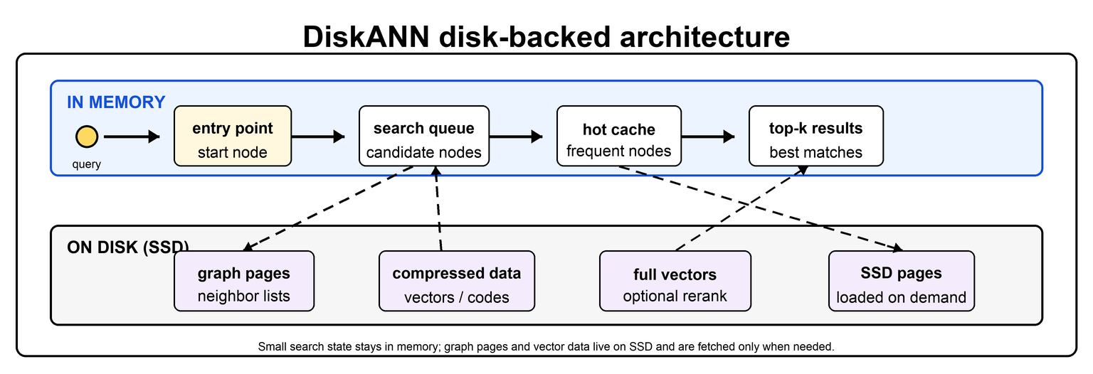
[Vamana/DiskANN](/user-guide/api-guides/indexing-guide/vamana) is designed for large-scale graph search where storage is part of the index design. Instead of treating disk as a slow overflow area, DiskANN-style indexes organize graph traversal and data layout so search can use SSD-backed storage more effectively. This makes them useful when an index is too large for memory but still needs high recall and low latency.
This is similar to the [locally partitioned indexes](/cuvs/getting-started/introduction/vector-database#locally-partitioned-indexes) architecture used by many vector databases. Local partitioning is useful for scaling storage, ingestion, and operations, but it does not reduce search work the way IVF or other similarity-aware routing structures can.
### Semantic Partitioning
Semantic partitioning groups similar vectors together so a query can search only the most relevant partitions. In vector search systems, semantic partitioning is usually based on [IVF-style architectures](#tree-based), where each partition is an inverted list selected by a coarse routing stage. The system pays an up-front clustering cost to preserve vector locality, then uses that locality to reduce query work.
At system scale, semantic partitioning can improve cache behavior and make larger indexes practical because hot partitions can remain in memory while less active partitions are searched less often. It is more complex to tune than hash partitioning because the number of partitions, assignment strategy, and number of partitions searched at query time all depend on dataset scale and distribution.
### Disk-based Indexes
Disk-based indexes are useful when the full dataset, graph, or compressed index does not fit comfortably in memory. They can make scale-up more cost efficient by using SSD capacity instead of keeping every vector and index structure in RAM, but they trade off some performance because disk access is slower and more variable than memory access.
Hash-partitioned indexes, also called blind-sharded indexes, are difficult to use efficiently from disk because each query usually needs to search every partition. If every partition may contain a nearest neighbor, then the system has to touch many files or segments at query time. That can make disk latency dominate the search.
Semantic partitioning can work better with disk when access patterns align with the partitions. A serving system can keep frequently used partitions in memory and leave less frequently used partitions on disk. This is most useful when queries repeatedly visit a subset of the vector space, because the hottest partitions can stay cached while colder partitions are loaded only when needed.
[Vamana/DiskANN](/user-guide/api-guides/indexing-guide/vamana) is designed for large-scale graph search where storage is part of the index design. Instead of treating disk as a slow overflow area, DiskANN-style indexes organize graph traversal and data layout so search can use SSD-backed storage more effectively. This makes them useful when an index is too large for memory but still needs high recall and low latency.
 ### Hybrid Architectures
Hash partitioning, semantic partitioning, graph-based indexing, and disk-backed storage are not mutually exclusive. A system can use hash partitioning for operational scale, semantic partitioning for similarity-aware routing, graph-based search for fast navigation inside selected partitions, and disk storage for colder data.
### Hybrid Architectures
Hash partitioning, semantic partitioning, graph-based indexing, and disk-backed storage are not mutually exclusive. A system can use hash partitioning for operational scale, semantic partitioning for similarity-aware routing, graph-based search for fast navigation inside selected partitions, and disk storage for colder data.
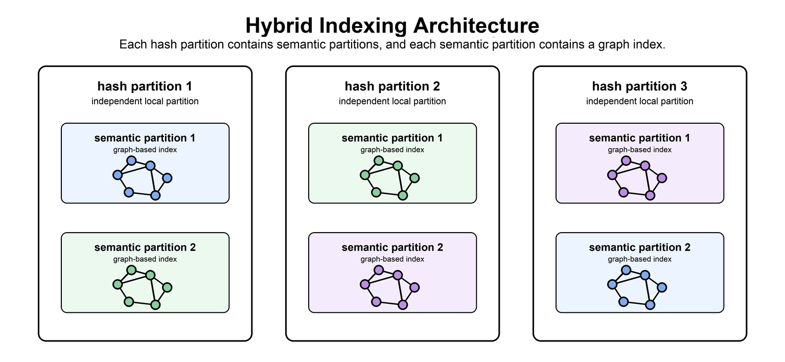 For example, a system might use hash partitions to distribute ingestion across nodes. Each hash partition can contain IVF partitions, and each IVF partition can contain a graph index such as CAGRA, HNSW, or Vamana. Search still fans out across hash partitions, but inside each partition the semantic and graph structures reduce the work.
Hybrid designs can also use memory and disk together. Hot semantic partitions or graph entry points can stay in memory, while colder graph pages or vector payloads live on disk. This keeps the serving architecture flexible while allowing the index to grow beyond memory-only limits.
### GPU Acceleration
GPU acceleration can help across the vector-search pipeline, not only during query search. Preprocessing steps such as quantization or dimensionality reduction, clustering steps such as k-means, index construction, refinement, and batched search can all benefit from GPU parallelism.
Some systems use GPUs only where they are most valuable. For example, a graph index can be built quickly on the GPU and converted to a CPU-searchable format such as HNSW, or a database can offload index builds to a GPU worker while keeping serving in its existing CPU runtime. These hybrid patterns let products shorten ingest or rebuild time without requiring every query-serving node to have a GPU.
For more integration details, see [Hybrid GPU-build and CPU-search](/user-guide/integration-patterns#hybrid-gpu-build-and-cpu-search) and [Offloaded index builds](/user-guide/integration-patterns#offloaded-index-builds).
## Choosing Index Types
Choosing an index starts with the workload, then narrows to the index family that best fits the target recall, latency, memory budget, build time, and deployment environment. The sections below give a practical starting point, compare the common options, and summarize when each index type is usually a good fit.
### Start with the Workload
The best index depends mostly on dataset size, vector dimensionality, recall target, and whether build time or query performance matters more.
| Workload | Good starting point |
| --- | --- |
| Tiny datasets, under 100K vectors | Use [brute-force](/user-guide/api-guides/indexing-guide/brute-force) or CPU [HNSW](/user-guide/api-guides/indexing-guide/cagra#interoperability-with-hnsw). A GPU index may not provide enough benefit to justify the extra complexity. |
| Small datasets, under 1M vectors | Use GPU [brute-force](/user-guide/api-guides/indexing-guide/brute-force) when exact results are acceptable and the vectors fit comfortably in memory. Use [HNSW](/user-guide/api-guides/indexing-guide/cagra#interoperability-with-hnsw) or [CAGRA](/user-guide/api-guides/indexing-guide/cagra) when lower latency is more important than exact recall. |
| Large datasets with fast ingest needs | Use [IVF-Flat](/user-guide/api-guides/indexing-guide/ivf-flat), [IVF-SQ](/user-guide/api-guides/indexing-guide/ivf-flat#ivf-sq-and-scalar-quantization), or [IVF-PQ](/user-guide/api-guides/indexing-guide/ivf-pq). These indexes partition the data and let you tune recall by searching more or fewer partitions. |
| Large datasets with high recall needs | Use [CAGRA](/user-guide/api-guides/indexing-guide/cagra) on GPU or [HNSW](/user-guide/api-guides/indexing-guide/cagra#interoperability-with-hnsw) on CPU. Graph indexes usually provide strong search quality, but take longer to build than IVF indexes. |
| Very large or disk-backed datasets | Use [Vamana/DiskANN](/user-guide/api-guides/indexing-guide/vamana) when the full dataset is too large to keep comfortably in memory. |
### Comparing Common Index Types
The table below compares common index families by the attributes that usually drive an initial design choice: build performance, search behavior, memory footprint, and the role each index plays in a larger system. Treat these as starting points rather than absolute rankings, because the best choice depends on the dataset, target recall, hardware, and deployment architecture.
| Algorithm | Build performance | Search performance | Memory footprint | Description |
| --- | --- | --- | --- | --- |
| [Brute-force](/user-guide/api-guides/indexing-guide/brute-force) | Fastest; no separate index build | Exact, but slow at large scale | Full vectors only | No index is built. Every query compares against every vector, so it is the simplest and most accurate baseline. |
| [HNSW](/user-guide/api-guides/indexing-guide/cagra#interoperability-with-hnsw) | Slower CPU graph construction | Very fast CPU search with strong recall | High due to graph links plus vectors | Builds a layered graph of nearby vectors. It is excellent for in-memory CPU search, but graph construction can be expensive. |
| [CAGRA](/user-guide/api-guides/indexing-guide/cagra) | Fast GPU graph construction | Very fast GPU ANN search | High due to graph links plus vectors | Fully GPU-accelerated graph-based algorithm. |
| [IVF-Flat](/user-guide/api-guides/indexing-guide/ivf-flat) | Fast partition training and assignment | Fast when probing a subset of partitions; exact within scanned partitions | Full vectors plus partition metadata | Partitions the dataset into coarse clusters, allowing the index to scale to larger datasets by searching only relevant partitions. Stores full-precision vectors. |
| [IVF-SQ](/user-guide/api-guides/indexing-guide/ivf-flat#ivf-sq-and-scalar-quantization) | Similar to IVF-Flat, with added quantization | Often faster than IVF-Flat due to lower memory bandwidth | Lower than IVF-Flat | IVF with scalar quantization. Vectors are compressed to reduce memory use and improve throughput with some recall tradeoff. |
| [IVF-PQ](/user-guide/api-guides/indexing-guide/ivf-pq) | More work than IVF-Flat because PQ codebooks are trained | Very memory-efficient; search speed depends on compression, probing, and refinement | Much lower than IVF-Flat or IVF-SQ | IVF with product quantization. Splits vectors into subvectors and stores compact codes, enabling much smaller indexes with a larger accuracy tradeoff than IVF-SQ. |
| [ScaNN](/user-guide/api-guides/indexing-guide/sca-nn) | Multi-stage build with partitioning and quantization | Strong recall and speed tradeoff | Usually reduced by quantization | Combines partitioning, quantization, and reranking to prune the search space while preserving result quality. |
| [Vamana/DiskANN](/user-guide/api-guides/indexing-guide/vamana) | Graph construction can be expensive | Excellent at very large scale, including SSD-backed search | Tuned for large memory or SSD-backed indexes | Builds a graph designed for large or disk-backed indexes, especially when the full dataset cannot fit comfortably in memory. |
### When to use each
Use [brute-force](/user-guide/api-guides/indexing-guide/brute-force) for exact baselines, small datasets, or validation.
Use locality-sensitive hashing when approximate bucket lookup is a good fit for the metric and recall target, or when evaluating hash-based candidate generation strategies.
Use [IVF-Flat](/user-guide/api-guides/indexing-guide/ivf-flat) when you want partition-based scaling while keeping full-precision vectors.
Use [IVF-SQ](/user-guide/api-guides/indexing-guide/ivf-flat#ivf-sq-and-scalar-quantization) when memory bandwidth or index size matters and a small recall tradeoff is acceptable.
Use [IVF-PQ](/user-guide/api-guides/indexing-guide/ivf-pq) when index size is the main bottleneck and stronger compression is worth additional tuning or reranking.
Use [HNSW](/user-guide/api-guides/indexing-guide/cagra#interoperability-with-hnsw) for high-quality CPU search when the index fits in memory.
Use [CAGRA](/user-guide/api-guides/indexing-guide/cagra) for high-throughput GPU search, fast GPU index construction, or hybrid workflows where a GPU-built graph is converted to HNSW for CPU search.
Use [ScaNN](/user-guide/api-guides/indexing-guide/sca-nn) when you want a tuned combination of partitioning, quantization, and reranking.
Use [Vamana/DiskANN](/user-guide/api-guides/indexing-guide/vamana) for very large datasets, especially when SSD-backed search is important, or hybrid workflows where a GPU-built graph is converted to CPU for DiskANN search.
## Conclusion
Vector search starts with a simple goal: find nearest neighbors. Indexes make that goal practical at scale by reducing vector footprint, reducing the number of distances, distributing work across partitions, using disk where memory is too costly, and accelerating expensive stages with GPUs.
Use brute force as the exact baseline, graph-based indexes when high-quality neighbor navigation is the best fit, IVF-partitioned indexes when similarity-aware partitioning helps reduce search work, and disk-oriented indexes when scale exceeds available memory. Compression, dimensionality reduction, reranking, partitioning, and GPU acceleration are additional tools that can improve memory use, build time, throughput, or recall once the basic index family is chosen.
In practice, start with the simplest index that can meet the target quality and latency, then tune search-time parameters before adding more build cost or system complexity.
For example, a system might use hash partitions to distribute ingestion across nodes. Each hash partition can contain IVF partitions, and each IVF partition can contain a graph index such as CAGRA, HNSW, or Vamana. Search still fans out across hash partitions, but inside each partition the semantic and graph structures reduce the work.
Hybrid designs can also use memory and disk together. Hot semantic partitions or graph entry points can stay in memory, while colder graph pages or vector payloads live on disk. This keeps the serving architecture flexible while allowing the index to grow beyond memory-only limits.
### GPU Acceleration
GPU acceleration can help across the vector-search pipeline, not only during query search. Preprocessing steps such as quantization or dimensionality reduction, clustering steps such as k-means, index construction, refinement, and batched search can all benefit from GPU parallelism.
Some systems use GPUs only where they are most valuable. For example, a graph index can be built quickly on the GPU and converted to a CPU-searchable format such as HNSW, or a database can offload index builds to a GPU worker while keeping serving in its existing CPU runtime. These hybrid patterns let products shorten ingest or rebuild time without requiring every query-serving node to have a GPU.
For more integration details, see [Hybrid GPU-build and CPU-search](/user-guide/integration-patterns#hybrid-gpu-build-and-cpu-search) and [Offloaded index builds](/user-guide/integration-patterns#offloaded-index-builds).
## Choosing Index Types
Choosing an index starts with the workload, then narrows to the index family that best fits the target recall, latency, memory budget, build time, and deployment environment. The sections below give a practical starting point, compare the common options, and summarize when each index type is usually a good fit.
### Start with the Workload
The best index depends mostly on dataset size, vector dimensionality, recall target, and whether build time or query performance matters more.
| Workload | Good starting point |
| --- | --- |
| Tiny datasets, under 100K vectors | Use [brute-force](/user-guide/api-guides/indexing-guide/brute-force) or CPU [HNSW](/user-guide/api-guides/indexing-guide/cagra#interoperability-with-hnsw). A GPU index may not provide enough benefit to justify the extra complexity. |
| Small datasets, under 1M vectors | Use GPU [brute-force](/user-guide/api-guides/indexing-guide/brute-force) when exact results are acceptable and the vectors fit comfortably in memory. Use [HNSW](/user-guide/api-guides/indexing-guide/cagra#interoperability-with-hnsw) or [CAGRA](/user-guide/api-guides/indexing-guide/cagra) when lower latency is more important than exact recall. |
| Large datasets with fast ingest needs | Use [IVF-Flat](/user-guide/api-guides/indexing-guide/ivf-flat), [IVF-SQ](/user-guide/api-guides/indexing-guide/ivf-flat#ivf-sq-and-scalar-quantization), or [IVF-PQ](/user-guide/api-guides/indexing-guide/ivf-pq). These indexes partition the data and let you tune recall by searching more or fewer partitions. |
| Large datasets with high recall needs | Use [CAGRA](/user-guide/api-guides/indexing-guide/cagra) on GPU or [HNSW](/user-guide/api-guides/indexing-guide/cagra#interoperability-with-hnsw) on CPU. Graph indexes usually provide strong search quality, but take longer to build than IVF indexes. |
| Very large or disk-backed datasets | Use [Vamana/DiskANN](/user-guide/api-guides/indexing-guide/vamana) when the full dataset is too large to keep comfortably in memory. |
### Comparing Common Index Types
The table below compares common index families by the attributes that usually drive an initial design choice: build performance, search behavior, memory footprint, and the role each index plays in a larger system. Treat these as starting points rather than absolute rankings, because the best choice depends on the dataset, target recall, hardware, and deployment architecture.
| Algorithm | Build performance | Search performance | Memory footprint | Description |
| --- | --- | --- | --- | --- |
| [Brute-force](/user-guide/api-guides/indexing-guide/brute-force) | Fastest; no separate index build | Exact, but slow at large scale | Full vectors only | No index is built. Every query compares against every vector, so it is the simplest and most accurate baseline. |
| [HNSW](/user-guide/api-guides/indexing-guide/cagra#interoperability-with-hnsw) | Slower CPU graph construction | Very fast CPU search with strong recall | High due to graph links plus vectors | Builds a layered graph of nearby vectors. It is excellent for in-memory CPU search, but graph construction can be expensive. |
| [CAGRA](/user-guide/api-guides/indexing-guide/cagra) | Fast GPU graph construction | Very fast GPU ANN search | High due to graph links plus vectors | Fully GPU-accelerated graph-based algorithm. |
| [IVF-Flat](/user-guide/api-guides/indexing-guide/ivf-flat) | Fast partition training and assignment | Fast when probing a subset of partitions; exact within scanned partitions | Full vectors plus partition metadata | Partitions the dataset into coarse clusters, allowing the index to scale to larger datasets by searching only relevant partitions. Stores full-precision vectors. |
| [IVF-SQ](/user-guide/api-guides/indexing-guide/ivf-flat#ivf-sq-and-scalar-quantization) | Similar to IVF-Flat, with added quantization | Often faster than IVF-Flat due to lower memory bandwidth | Lower than IVF-Flat | IVF with scalar quantization. Vectors are compressed to reduce memory use and improve throughput with some recall tradeoff. |
| [IVF-PQ](/user-guide/api-guides/indexing-guide/ivf-pq) | More work than IVF-Flat because PQ codebooks are trained | Very memory-efficient; search speed depends on compression, probing, and refinement | Much lower than IVF-Flat or IVF-SQ | IVF with product quantization. Splits vectors into subvectors and stores compact codes, enabling much smaller indexes with a larger accuracy tradeoff than IVF-SQ. |
| [ScaNN](/user-guide/api-guides/indexing-guide/sca-nn) | Multi-stage build with partitioning and quantization | Strong recall and speed tradeoff | Usually reduced by quantization | Combines partitioning, quantization, and reranking to prune the search space while preserving result quality. |
| [Vamana/DiskANN](/user-guide/api-guides/indexing-guide/vamana) | Graph construction can be expensive | Excellent at very large scale, including SSD-backed search | Tuned for large memory or SSD-backed indexes | Builds a graph designed for large or disk-backed indexes, especially when the full dataset cannot fit comfortably in memory. |
### When to use each
Use [brute-force](/user-guide/api-guides/indexing-guide/brute-force) for exact baselines, small datasets, or validation.
Use locality-sensitive hashing when approximate bucket lookup is a good fit for the metric and recall target, or when evaluating hash-based candidate generation strategies.
Use [IVF-Flat](/user-guide/api-guides/indexing-guide/ivf-flat) when you want partition-based scaling while keeping full-precision vectors.
Use [IVF-SQ](/user-guide/api-guides/indexing-guide/ivf-flat#ivf-sq-and-scalar-quantization) when memory bandwidth or index size matters and a small recall tradeoff is acceptable.
Use [IVF-PQ](/user-guide/api-guides/indexing-guide/ivf-pq) when index size is the main bottleneck and stronger compression is worth additional tuning or reranking.
Use [HNSW](/user-guide/api-guides/indexing-guide/cagra#interoperability-with-hnsw) for high-quality CPU search when the index fits in memory.
Use [CAGRA](/user-guide/api-guides/indexing-guide/cagra) for high-throughput GPU search, fast GPU index construction, or hybrid workflows where a GPU-built graph is converted to HNSW for CPU search.
Use [ScaNN](/user-guide/api-guides/indexing-guide/sca-nn) when you want a tuned combination of partitioning, quantization, and reranking.
Use [Vamana/DiskANN](/user-guide/api-guides/indexing-guide/vamana) for very large datasets, especially when SSD-backed search is important, or hybrid workflows where a GPU-built graph is converted to CPU for DiskANN search.
## Conclusion
Vector search starts with a simple goal: find nearest neighbors. Indexes make that goal practical at scale by reducing vector footprint, reducing the number of distances, distributing work across partitions, using disk where memory is too costly, and accelerating expensive stages with GPUs.
Use brute force as the exact baseline, graph-based indexes when high-quality neighbor navigation is the best fit, IVF-partitioned indexes when similarity-aware partitioning helps reduce search work, and disk-oriented indexes when scale exceeds available memory. Compression, dimensionality reduction, reranking, partitioning, and GPU acceleration are additional tools that can improve memory use, build time, throughput, or recall once the basic index family is chosen.
In practice, start with the simplest index that can meet the target quality and latency, then tune search-time parameters before adding more build cost or system complexity.