> For clean Markdown of any page, append .md to the page URL.
> For a complete documentation index, see https://docs.nvidia.com/cuvs/llms.txt.
> For full documentation content, see https://docs.nvidia.com/cuvs/llms-full.txt.
> For AI client integration (Claude Code, Cursor, etc.), connect to the MCP server at https://docs.nvidia.com/cuvs/_mcp/server.
# Methodologies
Vector search indexes should be compared by both search quality and performance. A fast index is not useful if it misses too many neighbors, and a high-recall index may not be practical if it is too slow to build or query. For index selection guidance, see [Vector Database](/cuvs/getting-started/introduction/vector-database).
This page describes how to make benchmark results comparable by using recall buckets, Pareto curves, and consistent reporting for build and search metrics. It also explains how these ideas apply to large datasets and points to cuVS Bench for reproducible benchmark runs.
## Pareto curves
Imagine every tuning run is a toy car. You want a car that is fast, but you also care how much work it took to build. If one car is both faster and easier to build than another car, the slower and harder-to-build car is not a useful choice. The cars that are not beaten this way form the Pareto curve.
For vector indexes, each tuning run is a point with [quality](#recall), build time, and search performance. A point is on the Pareto curve when no other run is better on the metric being compared without making another metric worse. Finding these points usually requires a parameter sweep or another hyperparameter optimization method.
 For each quality bucket, summarize build time by taking the points on the Pareto curve in that bucket and averaging their corresponding build times. This gives an expected build time for the quality window instead of forcing one run to represent the whole bucket.
## Recall
Recall measures how many exact nearest neighbors were returned by an approximate search. For one query, recall is the number of returned neighbors that also appear in the exact ground-truth result, divided by `k`. Across many queries, divide the total number of matched neighbors by `n_queries * k`.
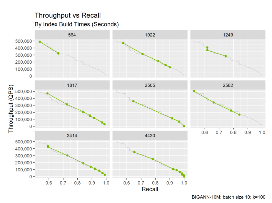
Index parameters control the recall and performance trade-off. The figure below shows eight indexes trained on the same data with different parameters. Higher recall often requires longer build times or slower searches, so reporting only the fastest or highest-recall run is not a fair comparison.
For each quality bucket, summarize build time by taking the points on the Pareto curve in that bucket and averaging their corresponding build times. This gives an expected build time for the quality window instead of forcing one run to represent the whole bucket.
## Recall
Recall measures how many exact nearest neighbors were returned by an approximate search. For one query, recall is the number of returned neighbors that also appear in the exact ground-truth result, divided by `k`. Across many queries, divide the total number of matched neighbors by `n_queries * k`.
Index parameters control the recall and performance trade-off. The figure below shows eight indexes trained on the same data with different parameters. Higher recall often requires longer build times or slower searches, so reporting only the fastest or highest-recall run is not a fair comparison.
 ## Fair comparisons
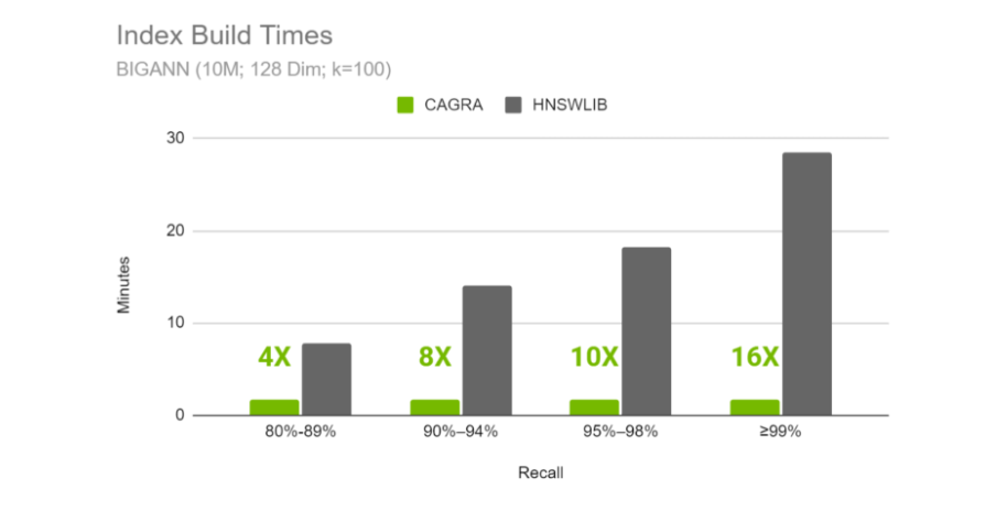
Compare latency, throughput, and build time only at similar recall levels. If two indexes are measured at different recall, the comparison mixes quality and speed into one number, and this is not a fair comparison.
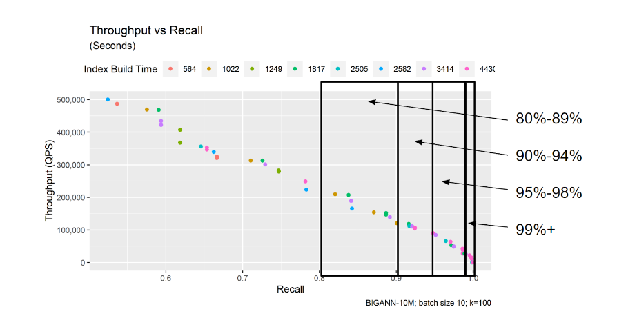
A practical approach is to group results into recall buckets:
| Recall bucket | Typical use |
| --- | --- |
| 80% - 89% | Fast exploratory search |
| 90% - 94% | Lower-latency approximate search |
| 95% - 98% | High-quality approximate search |
| 99%+ | Near-exact search |
## Fair comparisons
Compare latency, throughput, and build time only at similar recall levels. If two indexes are measured at different recall, the comparison mixes quality and speed into one number, and this is not a fair comparison.
A practical approach is to group results into recall buckets:
| Recall bucket | Typical use |
| --- | --- |
| 80% - 89% | Fast exploratory search |
| 90% - 94% | Lower-latency approximate search |
| 95% - 98% | High-quality approximate search |
| 99%+ | Near-exact search |
 This makes results easier to interpret. For example: "At 95% recall, model A builds 3x faster than model B, but model B has 2x lower latency."
 ## Large datasets
For database architecture terms, see the [Vector Database](/cuvs/getting-started/introduction/vector-database) guide. This page focuses on how to benchmark once the evaluation scope is clear: a standalone index, one local partition, a globally partitioned index, or the full database system.
Representative-sample tuning is appropriate when the benchmarked sample matches the unit that will actually be searched in production. For locally partitioned systems, that usually means tuning against the expected partition or segment size, not the full database size. For globally partitioned systems, tuning is more dependent on the full data distribution, so random samples need to be used carefully.
For a step-by-step workflow, see [Tuning Indexes](/cuvs/getting-started/introduction/tuning-indexes).
## Methodology summary
- Define the scope, dataset, distance metric, `k`, batch size, filters, hardware, and concurrency before comparing results.
- Generate exact ground truth, sweep or tune build and search parameters, group results into recall buckets, and compare Pareto points within each bucket.
- Report recall, latency, throughput, build time, and memory (if needed) together so quality and performance are not separated from the cost of achieving them.
cuVS provides [cuVS Bench](/cuvs/user-guide/benchmarking-guide/cu-vs-bench-tool/introduction) for reproducible benchmarks that follow these methodologies and produce comparable outputs across datasets, algorithms, and hardware.
## Large datasets
For database architecture terms, see the [Vector Database](/cuvs/getting-started/introduction/vector-database) guide. This page focuses on how to benchmark once the evaluation scope is clear: a standalone index, one local partition, a globally partitioned index, or the full database system.
Representative-sample tuning is appropriate when the benchmarked sample matches the unit that will actually be searched in production. For locally partitioned systems, that usually means tuning against the expected partition or segment size, not the full database size. For globally partitioned systems, tuning is more dependent on the full data distribution, so random samples need to be used carefully.
For a step-by-step workflow, see [Tuning Indexes](/cuvs/getting-started/introduction/tuning-indexes).
## Methodology summary
- Define the scope, dataset, distance metric, `k`, batch size, filters, hardware, and concurrency before comparing results.
- Generate exact ground truth, sweep or tune build and search parameters, group results into recall buckets, and compare Pareto points within each bucket.
- Report recall, latency, throughput, build time, and memory (if needed) together so quality and performance are not separated from the cost of achieving them.
cuVS provides [cuVS Bench](/cuvs/user-guide/benchmarking-guide/cu-vs-bench-tool/introduction) for reproducible benchmarks that follow these methodologies and produce comparable outputs across datasets, algorithms, and hardware.