Getting Started
Overview
NVIDIA Data Loading Library (DALI) is a collection of highly optimized building blocks and an execution engine that accelerates the data pipeline for computer vision and audio deep learning applications.
Input and augmentation pipelines provided by Deep Learning frameworks fit typically into one of two categories:
fast, but inflexible - written in C++, they are exposed as a single monolithic Python object with very specific set and ordering of operations it provides
slow, but flexible - set of building blocks written in either C++ or Python, that can be used to compose arbitrary data pipelines that end up being slow. One of the biggest overheads for this type of data pipelines is Global Interpreter Lock (GIL) in Python. This forces developers to use multiprocessing, complicating the design of efficient input pipelines.
DALI stands out by providing both performance and flexibility of accelerating different data pipelines. It achieves that by exposing optimized building blocks which are executed using simple and efficient engine, and enabling offloading of operations to GPU (thus enabling scaling to multi-GPU systems).
It is a single library, that can be easily integrated into different deep learning training and inference applications.
DALI offers ease-of-use and flexibility across GPU enabled systems with direct framework plugins, multiple input data formats, and configurable graphs. DALI can help achieve overall speedup on deep learning workflows that are bottlenecked on I/O pipelines due to the limitations of CPU cycles. Typically, systems with high GPU to CPU ratio (such as Amazon EC2 P3.16xlarge, NVIDIA DGX1-V or NVIDIA DGX-2) are constrained on the host CPU, thereby under-utilizing the available GPU compute capabilities. DALI significantly accelerates input processing on such dense GPU configurations to achieve the overall throughput.
Pipeline
At the core of data processing with DALI lies the concept of a data processing pipeline. It is composed of multiple operations connected in a directed graph and contained in an object of class class nvidia.dali.Pipeline. This class provides functions necessary for defining, building and running data processing pipelines.
[1]:
from nvidia.dali.pipeline import Pipeline
Defining the Pipeline
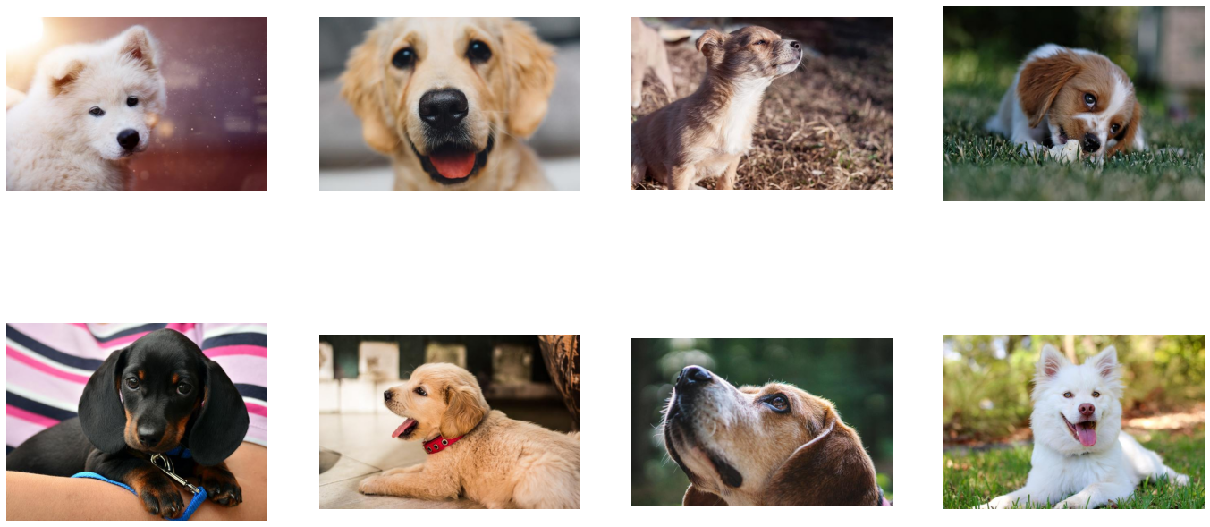
Let us start with defining a very simple pipeline for a classification task determining whether a picture contains a dog or a kitten. We prepared a directory structure containing pictures of dogs and kittens in our repository.
Our simple pipeline will read images from this directory, decode them and return (image, label) pairs.
The easiest way to create a pipieline is by using the pipeline_def decorator. In the simple_pipeline function we define the operations to be performed and the flow of the computation between them.
Use
fn.readers.fileto read jpegs (encoded images) and labels from the hard drive.Use the
fn.decoders.imageoperation to decode images from jpeg to RGB.Specify which of the intermediate variables should be returned as the outputs of the pipeline.
For more information about pipeline_def look to the documentation.
[2]:
from nvidia.dali import pipeline_def
import nvidia.dali.fn as fn
import nvidia.dali.types as types

image_dir = "data/images"
max_batch_size = 8


@pipeline_def
def simple_pipeline():
    jpegs, labels = fn.readers.file(file_root=image_dir)
    images = fn.decoders.image(jpegs, device="cpu")

    return images, labels
Building the Pipeline
In order to use the pipeline defined with simple_pipeline, we need to create and build it. This is achieved by calling simple_pipeline, which creates an instance of the pipeline. Then we call build on this newly created instance:
[3]:
pipe = simple_pipeline(batch_size=max_batch_size, num_threads=1, device_id=0)
pipe.build()
Notice that decorating a function with pipeline_def adds new named arguments to it. They can be used to control various aspects of the pipeline, such as:
max batch size,
number of threads used to perform computation on the CPU,
which GPU device to use (pipeline created with
simple_pipelinedoes not yet use GPU for compute though),seed for random number generation.
For more information about Pipeline arguments you can look to Pipeline documentation.
Running the Pipeline
After the pipeline is built, we can run it to get a batch of results.
[4]:
pipe_out = pipe.run()
print(pipe_out)
(TensorListCPU(
    [[[[255 255 255]
      [255 255 255]
      ...
      [ 86  46  55]
      [ 86  46  55]]

     [[255 255 255]
      [255 255 255]
      ...
      [ 86  46  55]
      [ 86  46  55]]

     ...

     [[158 145 154]
      [158 147 155]
      ...
      [ 93  38  41]
      [ 93  38  41]]

     [[157 145 155]
      [158 146 156]
      ...
      [ 93  38  41]
      [ 93  38  41]]]


    [[[ 69  77  80]
      [ 69  77  80]
      ...
      [ 97 105 108]
      [ 97 105 108]]

     [[ 69  77  80]
      [ 70  78  81]
      ...
      [ 97 105 108]
      [ 97 105 108]]

     ...

     [[199 203 206]
      [199 203 206]
      ...
      [206 210 213]
      [206 210 213]]

     [[199 203 206]
      [199 203 206]
      ...
      [206 210 213]
      [206 210 213]]]


    ...


    [[[ 26  28  25]
      [ 26  28  25]
      ...
      [ 34  39  33]
      [ 34  39  33]]

     [[ 26  28  25]
      [ 26  28  25]
      ...
      [ 34  39  33]
      [ 34  39  33]]

     ...

     [[ 35  46  30]
      [ 36  47  31]
      ...
      [114  99 106]
      [127 114 121]]

     [[ 35  46  30]
      [ 35  46  30]
      ...
      [107  92  99]
      [112  97 102]]]


    [[[182 185 132]
      [180 183 128]
      ...
      [ 98 103   9]
      [ 97 102   8]]

     [[180 183 130]
      [179 182 127]
      ...
      [ 93  98   4]
      [ 91  96   2]]

     ...

     [[ 69 111  71]
      [ 68 111  66]
      ...
      [147 159 121]
      [148 163 124]]

     [[ 64 109  68]
      [ 64 110  64]
      ...
      [113 123  88]
      [104 116  80]]]],
    dtype=DALIDataType.UINT8,
    layout="HWC",
    num_samples=8,
    shape=[(427, 640, 3),
           (427, 640, 3),
           (425, 640, 3),
           (480, 640, 3),
           (485, 640, 3),
           (427, 640, 3),
           (409, 640, 3),
           (427, 640, 3)]), TensorListCPU(
    [[0]
     [0]
     [0]
     [0]
     [0]
     [0]
     [0]
     [0]],
    dtype=DALIDataType.INT32,
    num_samples=8,
    shape=[(1,), (1,), (1,), (1,), (1,), (1,), (1,), (1,)]))
The output of the pipeline, which we saved to pipe_out variable, is a tuple of 2 elements (as expected - we specified 2 outputs in simple_pipeline function). Both of these elements are TensorListCPU objects - each containing a list of CPU tensors.
In order to show the results (just for debugging purposes - during the actual training we would not do that step, as it would make our batch of images do a round trip from GPU to CPU and back) we can send our data from DALI’s Tensor to NumPy array. Not every TensorList can be accessed that way though - TensorList is more general than NumPy array and can hold tensors with different shapes. In order to check whether we can send it to NumPy directly, we can call the is_dense_tensor
function of TensorList
[5]:
images, labels = pipe_out
print("Images is_dense_tensor: " + str(images.is_dense_tensor()))
print("Labels is_dense_tensor: " + str(labels.is_dense_tensor()))
Images is_dense_tensor: False
Labels is_dense_tensor: True
As it turns out, TensorList containing labels can be represented by a tensor, while the TensorList containing images cannot.
Let us see, what is the shape and contents of returned labels.
[6]:
print(labels)
TensorListCPU(
    [[0]
     [0]
     [0]
     [0]
     [0]
     [0]
     [0]
     [0]],
    dtype=DALIDataType.INT32,
    num_samples=8,
    shape=[(1,), (1,), (1,), (1,), (1,), (1,), (1,), (1,)])
In order to see the images, we will need to loop over all tensors contained in TensorList, accessed with its at method.
[7]:
import matplotlib.gridspec as gridspec
import matplotlib.pyplot as plt

%matplotlib inline


def show_images(image_batch):
    columns = 4
    rows = (max_batch_size + 1) // (columns)
    fig = plt.figure(figsize=(24, (24 // columns) * rows))
    gs = gridspec.GridSpec(rows, columns)
    for j in range(rows * columns):
        plt.subplot(gs[j])
        plt.axis("off")
        plt.imshow(image_batch.at(j))
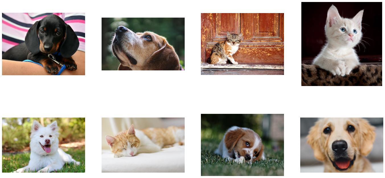
[8]:
show_images(images)
Adding Augmentations
Random Shuffle
As we can see from the example above, the first batch of images returned by our pipeline contains only dogs. That is because we did not shuffle our dataset, and so fn.readers.file returns images in lexicographic order.
Let us make a new pipeline, that will change that.
[9]:
@pipeline_def
def shuffled_pipeline():
    jpegs, labels = fn.readers.file(file_root=image_dir, random_shuffle=True, initial_fill=21)
    images = fn.decoders.image(jpegs, device="cpu")

    return images, labels
We made 2 changes to the simple_pipeline to obtain the shuffled_pipeline - we added 2 arguments to the fn.readers.file operation
random_shuffleenables shuffling of images in the reader. Shuffling is performed by using a buffer of images read from disk. When the reader is asked to provide the next image, it randomly selects an image from the buffer, outputs it and immediately replaces that spot in the buffer with a freshly read image.initial_fillsets the capacity of the buffer. The default value of this parameter (1000), well suited for datasets containing thousands of examples, is too big for our very small dataset, which contains only 21 images. This could result in frequent duplicates in the returned batch. That is why in this example we set it to the size of our dataset.
Let us test the result of this modification.
[10]:
pipe = shuffled_pipeline(batch_size=max_batch_size, num_threads=1, device_id=0, seed=1234)
pipe.build()
[11]:
pipe_out = pipe.run()
images, labels = pipe_out
show_images(images)
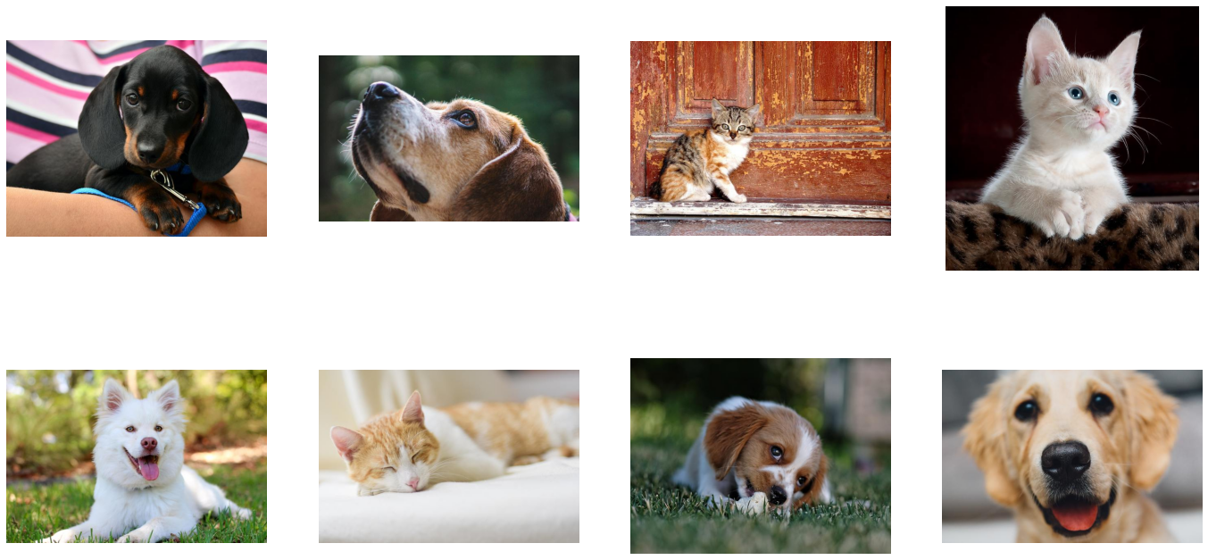
Now the images returned by the pipeline are shuffled properly.
Augmentations
DALI can not only read images from disk and batch them into tensors, it can also perform various augmentations on those images to improve Deep Learning training results.
One example of such augmentations is rotation. Let us make a new pipeline, which rotates the images before outputting them.
[12]:
@pipeline_def
def rotated_pipeline():
jpegs, labels = fn.readers.file(file_root=image_dir, random_shuffle=True, initial_fill=21)
images = fn.decoders.image(jpegs, device="cpu")
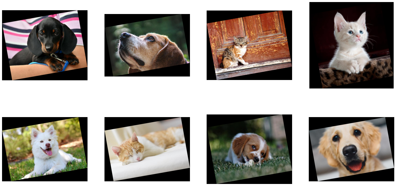
rotated_images = fn.rotate(images, angle=10.0, fill_value=0)
return rotated_images, labels
To do that, we added a new operation to our pipeline: fn.rotate.
As we can see in the documentation, rotate can take multiple arguments, but only one of them beyond input is required - angle tells the operator how much it should rotate images. We also specified fill_value to better visualise the results.
Let us test the newly created pipeline:
[13]:
pipe = rotated_pipeline(batch_size=max_batch_size, num_threads=1, device_id=0, seed=1234)
pipe.build()
[14]:
pipe_out = pipe.run()
images, labels = pipe_out
show_images(images)
Tensors as Arguments and Random Number Generation
Rotating every image by 10 degrees is not that interesting. To make a meaningful augmentation, we would like an operator that rotates our images by a random angle in a given range.
Rotate’s angle parameter can accept float or float tensor types of values. The second option, float tensor, enables us to feed the operator with different rotation angles for every image, via a tensor produced by other operation.
Random number generators are examples of operations that one can use with DALI. Let us use fn.random.uniform to make a pipeline that rotates images by a random angle.
NOTE
Keep in mind, that every time you pass an output of a DALI operator to another as a named keyword argument that data must be placed on the CPU. In the example below, we use the output of
random.uniform(which has a default device=’cpu’) asanglekeyword argument torotate.Such arguments in DALI are called “argument inputs”. More information about them can be found in the pipeline documentation section.
Regular inputs (non-named, positional ones) do not have such constraints and can use either CPU or GPU data, as show below.
[15]:
@pipeline_def
def random_rotated_pipeline():
jpegs, labels = fn.readers.file(file_root=image_dir, random_shuffle=True, initial_fill=21)
images = fn.decoders.image(jpegs, device="cpu")
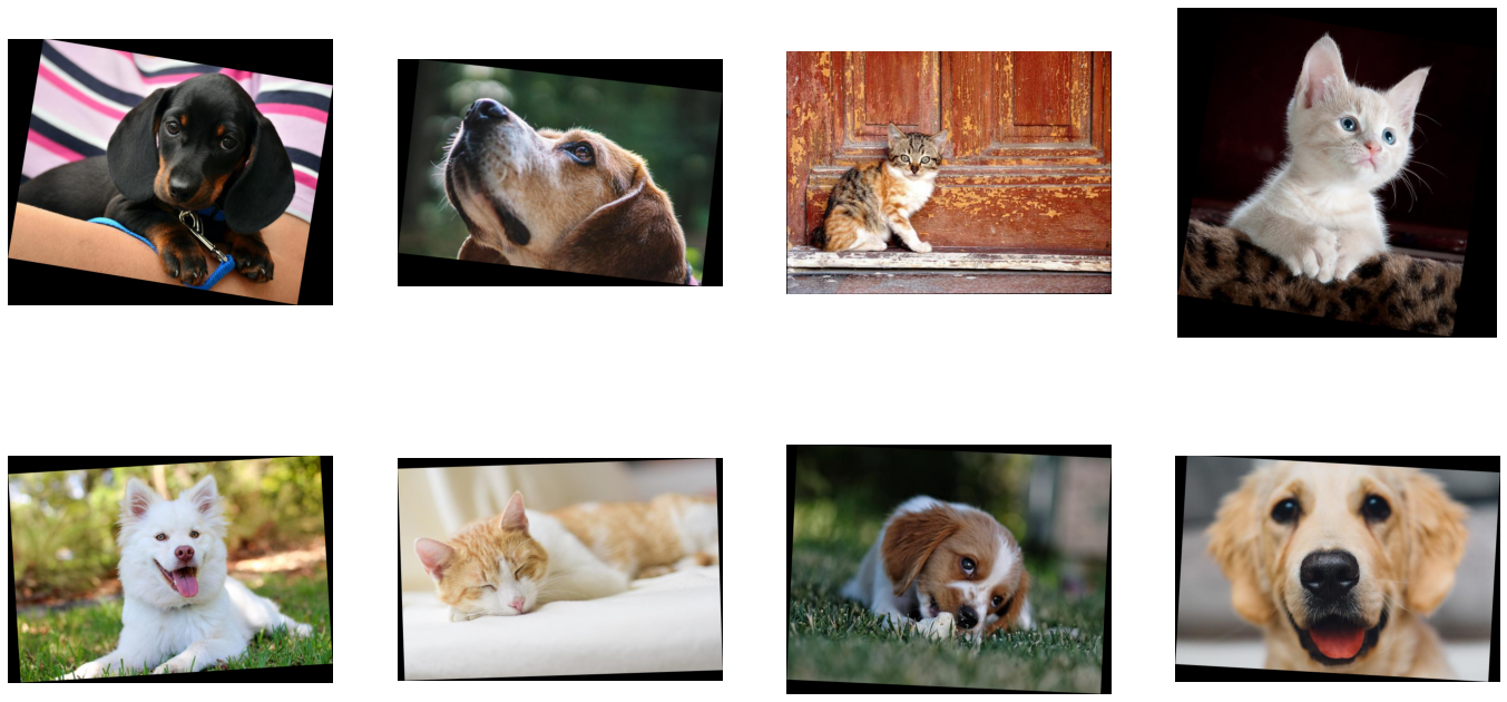
angle = fn.random.uniform(range=(-10.0, 10.0))
rotated_images = fn.rotate(images, angle=angle, fill_value=0)
return rotated_images, labels
This time, instead of providing a fixed value for the angle argument, we set it to the output of the fn.random.uniform operator.
Let us check the result:
[16]:
pipe = random_rotated_pipeline(batch_size=max_batch_size, num_threads=1, device_id=0, seed=1234)
pipe.build()
[17]:
pipe_out = pipe.run()
images, labels = pipe_out
show_images(images)

This time, the rotation angle is randomly selected from a value range.
Adding GPU Acceleration
DALI offers access to GPU accelerated operators, that can increase the speed of the input and augmentation pipeline and let it scale to multi-GPU systems.
Copying Tensors to GPU
Let us modify the previous example of the random_rotated_pipeline to use the GPU for the rotation.
[18]:
@pipeline_def
def random_rotated_gpu_pipeline():
    jpegs, labels = fn.readers.file(file_root=image_dir, random_shuffle=True, initial_fill=21)
    images = fn.decoders.image(jpegs, device="cpu")
    angle = fn.random.uniform(range=(-10.0, 10.0))
    rotated_images = fn.rotate(images.gpu(), angle=angle, fill_value=0)

    return rotated_images, labels
In order to tell DALI that we want to use the GPU, we needed to make only one change to the pipeline. We changed input to the rotate operation from images, which is a tensor on the CPU, to images.gpu() which copies it to the GPU.
[19]:
pipe = random_rotated_gpu_pipeline(batch_size=max_batch_size, num_threads=1, device_id=0, seed=1234)
pipe.build()
[20]:
pipe_out = pipe.run()
print(pipe_out)
(TensorListGPU(
    [[[[0 0 0]
      [0 0 0]
      ...
      [0 0 0]
      [0 0 0]]

     [[0 0 0]
      [0 0 0]
      ...
      [0 0 0]
      [0 0 0]]

     ...

     [[0 0 0]
      [0 0 0]
      ...
      [0 0 0]
      [0 0 0]]

     [[0 0 0]
      [0 0 0]
      ...
      [0 0 0]
      [0 0 0]]]


    [[[0 0 0]
      [0 0 0]
      ...
      [0 0 0]
      [0 0 0]]

     [[0 0 0]
      [0 0 0]
      ...
      [0 0 0]
      [0 0 0]]

     ...

     [[0 0 0]
      [0 0 0]
      ...
      [0 0 0]
      [0 0 0]]

     [[0 0 0]
      [0 0 0]
      ...
      [0 0 0]
      [0 0 0]]]


    ...


    [[[0 0 0]
      [0 0 0]
      ...
      [0 0 0]
      [0 0 0]]

     [[0 0 0]
      [0 0 0]
      ...
      [0 0 0]
      [0 0 0]]

     ...

     [[0 0 0]
      [0 0 0]
      ...
      [0 0 0]
      [0 0 0]]

     [[0 0 0]
      [0 0 0]
      ...
      [0 0 0]
      [0 0 0]]]


    [[[0 0 0]
      [0 0 0]
      ...
      [0 0 0]
      [0 0 0]]

     [[0 0 0]
      [0 0 0]
      ...
      [0 0 0]
      [0 0 0]]

     ...

     [[0 0 0]
      [0 0 0]
      ...
      [0 0 0]
      [0 0 0]]

     [[0 0 0]
      [0 0 0]
      ...
      [0 0 0]
      [0 0 0]]]],
    dtype=DALIDataType.UINT8,
    layout="HWC",
    num_samples=8,
    shape=[(583, 710, 3),
           (477, 682, 3),
           (482, 642, 3),
           (761, 736, 3),
           (467, 666, 3),
           (449, 654, 3),
           (510, 662, 3),
           (463, 664, 3)]), TensorListCPU(
    [[0]
     [0]
     [1]
     [1]
     [0]
     [1]
     [0]
     [0]],
    dtype=DALIDataType.INT32,
    num_samples=8,
    shape=[(1,), (1,), (1,), (1,), (1,), (1,), (1,), (1,)]))
pipe_out still contains 2 TensorLists, but this time the first output, result of the rotate operation, is on the GPU. We cannot access contents of TensorListGPU directly from the CPU, so in order to visualize the result we need to copy it to the CPU by using as_cpu method.
[21]:
images, labels = pipe_out
show_images(images.as_cpu())
Important Notice
DALI does not support moving the data from the GPU to the CPU within the pipeline. That is why a CPU operation cannot follow a GPU one.
Hybrid Decoding
Sometimes, especially for higher resolution images, decoding images stored in JPEG format may become a bottleneck. To address this problem, nvJPEG and nvJPEG2000 libraries were developed. They split the decoding process between CPU and GPU, significantly reducing the decoding time.
Specifying “mixed” device parameter in fn.decoders.image enables nvJPEG and nvJPEG2000 support. Other file formats are still decoded on the CPU.
[22]:
@pipeline_def
def hybrid_pipeline():
    jpegs, labels = fn.readers.file(file_root=image_dir, random_shuffle=True, initial_fill=21)
    images = fn.decoders.image(jpegs, device="mixed")

    return images, labels
fn.decoders.image with device=mixed uses a hybrid approach of computation that employs both the CPU and the GPU. This means that it accepts CPU inputs, but returns GPU outputs. That is why images objects returned from the pipeline are of type TensorListGPU.
[23]:
pipe = hybrid_pipeline(batch_size=max_batch_size, num_threads=1, device_id=0, seed=1234)
pipe.build()
[24]:
pipe_out = pipe.run()
images, labels = pipe_out
show_images(images.as_cpu())
Let us compare the speed of fn.decoders.image for ‘cpu’ and ‘mixed’ backends by measuring speed of shuffled_pipeline and hybrid_pipeline with 4 CPU threads.
[25]:
from timeit import default_timer as timer

test_batch_size = 64


def speedtest(pipeline, batch, n_threads):
    pipe = pipeline(batch_size=batch, num_threads=n_threads, device_id=0)
    pipe.build()
    # warmup
    for i in range(5):
        pipe.run()
    # test
    n_test = 20
    t_start = timer()
    for i in range(n_test):
        pipe.run()
    t = timer() - t_start
    print("Speed: {} imgs/s".format((n_test * batch) / t))
[26]:
speedtest(shuffled_pipeline, test_batch_size, 4)
Speed: 2597.527149961429 imgs/s
[27]:
speedtest(hybrid_pipeline, test_batch_size, 4)
Speed: 5828.851662794091 imgs/s
As we can see, using GPU accelerated decoding resulted in significant speedup.