
This sample demonstrates the basic techniques for using DirectCompute to process images as part of a 3D rendering pipeline. Through a series of Compute shader passes, we convert an input image into a 'summed area table' (SAT) which can then be used by a post-processing shader to simulate basic depth-of-field.
This sample has the following app-specific controls:
| Device | Input | Result |
|---|---|---|
| mouse | Left-Click Drag | Rotate the view |
| keyboard | Arrow Keys | Translate the view left/right/forward/back |
| W/S | Translate the view forward/back | |
| A/D | Translate the view left/right | |
| TAB | Toggle the HUD | |
| F1 | Toggle help display | |
| F2 | Toggle the Test mode HUD | |
| gamepad | Right ThumbStick | Rotate the camera |
| Left ThumbStick | Move forward/backward, Slide left/right |
DirectCompute provides programmers with a tremendous amount of flexibility in how work is scheduled and organized across GPU cores, allowing them to exploit synergies between the processing of adjacent pixels which would be otherwise impossible with a traditional Pixel Shader approach. By allowing threads within a single Dispatch to communicate with one-another through Shared Memory which is visible only to threads in that dispatch, parallelism can be exploited to avoid redundant memory access and computation.
In other words, by performing filtering using DirectCompute, we can take advantage of locality to read and process data in a more parallel and efficient manner.
The "prefix sum" algorithm is an excellent example of this capability. There are many cases where one might want to compute the sum of a list of elements, or of some sub-set of that list. A traditional serial approach would involve walking over the list, adding each element to the running sum and storing the intermediate value in an output array. Unfortunately, this requires the processor to read in only a single value at a time (with potential caching) and requires a number of operations proportional to the number of elements in the array.
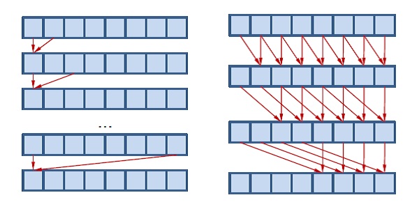
Figure 1. The serial (left) prefix-sum approach requires O(N) passes, while the parallel (right) approach only needs O(log2(N)) because it spreads the work over multiple threads.
However, with the use of shared memory, a multi-threaded workload such as a DirectCompute dispatch can schedule this work so that it can be done in a fraction of the cycle time. Although the amount of work being done is O(N) in both cases, the parallelism effectively reduces the workload to O(log(N)).
The Summed Area Table (SAT) is a transformation of some rectangular data set (like an image) such that every entry in the table equals the value of its corresponding source entry, plus all entries below and to the left of it. Thus, the values are constantly increasing from the bottom-left corner to the top-right corner. This property can, in turn, be exploited to determine the average value of the source data over an arbitrary rectangular area in constant time by differencing the values of the SAT at each corner, and then dividing by the total area of the region in question.
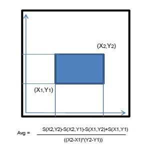
Figure 2. Since the values of a SAT pixel are based on all those below and to the left of it, you can quickly compute the average value over an arbitrary rectangular area with only four samples.
Since this averaging can be done in constant time and with a fixed number of texture samples, this approach is tremendously advantageous for applications where one needs to arbitrarily low-pass filter an image at varying kernel widths quickly. Furthermore, since it is essentially a 2-dimensional prefix sum, readily lends itself towards efficient computation using the GPU and Compute shaders.
Depth of Field (DoF) is an artifact of physical cameras and lenses (including the human eye) derived from the fact that the aperture through which light passes from the lens to the imaging plane is not ideal, so that there is actually a range of angles through which each point in the image can see the outside world. This effect is often subtle, but crucial to rendering truly photo-realistic scenes, as it is a part of every single physical camera in the real world. Furthermore, it is often used to dramatic effect to frame a scene, or draw the viewer's attention to a specific region, and clearly demark other sections as foreground or background.
The specific mechanics behind depth-of-field effects are beyond the scope of this sample; however, the general idea is that there is a single focal depth in the world for a given lens/aperture/image plane configuration where everything will be perfectly in focus, as if through a pin-hole camera. Surrounding that point is a focal range where the blur radius is smaller than the image medium's ability to resolve individual details (such as the size of a single pixel). Beyond that, objects will have multiple paths through the lens-aperture-image system which will cause them to appear blurred, becoming part of either foreground (nearer than the focal range) or background (further than the focal range).
We take advantage of the flexibility of summed-area tables and their amenability to GPU computation to quickly and efficiently approximate blur among foreground and background objects. Our rendering pipeline can be split into three stages:
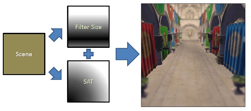
Figure 3. An overview of the SAT Depth-of-Field pipeline
The Summed-Area Table is generated by running the input image through a chain of Compute kernels, each one doing a portion of the sum operation. We begin by down-sampling the input by a factor of 2 -- this dramatically reduces memory and computation workload, and doesn't affect output quality much, since blur factors being used are much larger than a 2x2 pixel footprint where detail would be lost.
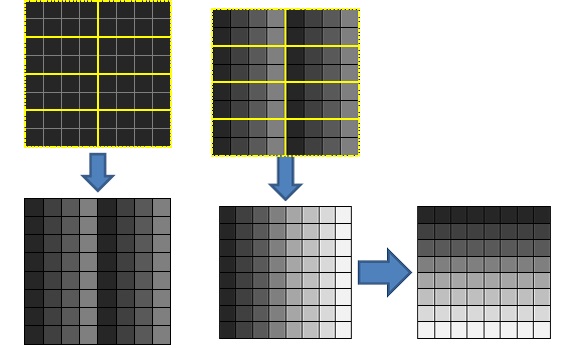
Figure 4. The first pass of the SAT algorithm: partial sum (left) and offset+transpose (right). Running this again on its own output will give us a SAT for the input image
From there, we perform a "partial prefix sum" on the image, issuing a dispatch which covers the entire image where each group computes a parallel prefix sum horizontally for each row that it covers. This output is then then fed to a second kernel, which computes the offset for each work group by summing the final element of each block to the left of the current group horizontally from the previous pass, giving the total amount that each value in that block must be offset to turn it into a proper global prefix-sum for the row.
Finally, this second pass transposes the pixel coordinates, swapping the x and y coordinates before output. This allows us to run the same shaders for both parts of the separable pass, and can preserve some advantageous texture access qualities by favoring reads across a row. By running the Sum and Offset/Transpose passes twice on the data, we end up with a complete summed-area table for the original image.
As the last stage, we feed both the original scene rendering (along with its Z-buffer) and the computed SAT into a post-process shader which produces the resultant image. We use the Z-buffer data to compute the size of the blur at each pixel:
Figure 5. Three overlapping boxes work well to approximate a smoother filter for larger kernels.
For large blur radii, the box-like nature of the SAT sample area can lead to undesirable artifacts; for this reason, we actually sample the SAT over three different areas (Rx0.5*R, 0.75*Rx0.75*R, and 0.5*RxR) and then combine them to approximate something closer to a Gaussian.
This approach provides continue real-time arbitrary filtering over very large areas with minimal up-front cost. There are some limitations to this approach, however.
First, the summed-area table approach can become hampered by precision issues if averages are taken over exceptionally large areas, or if the source data contains very high dynamic range values. Furthermore, since the SAT increases with the number of pixels, this problem can be exacerbated for very large framebuffers. There are ways around this, such as placing the "offset" values into a separate, lower resolution SAT, however they break naive interpolation and thus add more work to the shader and GPU.
Second, though the results are convincing in certain circumstances, the approach does not correctly approximate Depth of Field in scenes with a great deal of depth complexity. Depth-of-Field is actually a "scatter" effect -- an object out of focus will actually contribute to adjacent (non-occluded) pixels -- rather than a "gather" effect. Because of this, taking the blurred version of surrounding pixels is not correct if those pixels are either in focus or part of the foreground.
This problem cannot be completely avoided with the method suggested here; however, it can be greatly mitigated by creating two SATs: one for foreground objects, and one for background objects. Each SAT would be generated from a filtered version of the input image which only contained values for pixels in its assigned range band, and black everywhere else (meaning that those pixels would not contribute to the SAT). One would also have to add a "coverage" value to the alpha channel to distinguish between "empty" pixels and actual "black" ones, and then use that total value instead of the analytic area when computing the average of a summed area; however, this would be at minimal additional cost, given that we are already storing a four-channel format texture.
The (revised) Sponza Atrium model is generously provided to the public domain by Crytek.

NVIDIA® GameWorks™ Documentation Rev. 1.0.220830 ©2014-2022. NVIDIA Corporation and affiliates. All Rights Reserved.