
An OptiX context provides an interface for controlling the setup and subsequent launch of the ray tracing engine. Contexts are created with the rtContextCreate function. A context object encapsulates all OptiX resources -- textures, geometry, user-defined programs, etc. The destruction of a context, via the rtContextDestroy function, will clean up all of these resources and invalidate any existing handles to them.
rtContextLaunch{1,2,3}D serves as an entry point to ray engine computation. The launch function takes an entry point parameter, discussed in Section 3.1.1, as well as one, two or three grid dimension parameters. The dimensions establish a logical computation grid. Upon a call to rtContextLaunch, any necessary preprocessing is performed and then the ray generation program associated with the provided entry point index is invoked once per computational grid cell. The launch precomputation includes state validation and, if necessary, acceleration structure generation and kernel compilation. Output from the launch is passed back via OptiX buffers, typically but not necessarily of the same dimensionality as the computation grid.
RTcontext context;
rtContextCreate( &context );
unsigned int entry_point = ...;
unsigned int width = ...;
unsigned int height = ...;
// Set up context state and scene description
...
rtContextLaunch2D( entry_point, width, height );
rtContextDestroy( context );
While multiple contexts can be active at one time in limited cases, this is usually unnecessary as a single context object can leverage multiple hardware devices. The devices to be used can be specified with rtContextSetDevices. By default, the highest compute capable set of compatible OptiX-capable devices is used. The following set of rules is used to determine device compatibility. These rules could change in the future. If incompatible devices are selected an error is returned from rtContextSetDevices.
Each context may have multiple computation entry points. A context entry point is associated with a single ray generation program as well as an exception program. The total number of entry points for a given context can be set with rtContextSetEntryPointCount. Each entry point's associated programs are set and queried by rtContext{Set|Get}RayGenerationProgram and rtContext{Set|Get}ExceptionProgram. Each entry point must be assigned a ray generation program before use; however, the exception program is an optional program that allows users to specify behavior upon various error conditions. The multiple entry point mechanism allows switching between multiple rendering algorithms as well as efficient implementation of techniques such as multi-pass rendering on a single OptiX context.
RTcontext context = ...;
rtContextSetEntryPointCount( context, 2 );

RTprogram pinhole_camera = ...;
RTprogram thin_lens_camera = ...;
RTprogram exception = ...;

rtContextSetRayGenerationProgram( context, 0,
				  pinhole_camera );
rtContextSetRayGenerationProgram( context, 1,
				  thin_lens_camera );
rtContextSetExceptionProgram( context, 0, exception );
rtContextSetExceptionProgram( context, 1, exception );
OptiX supports the notion of ray types, which is useful to distinguish between rays that are traced for different purposes. For example, a renderer might distinguish between rays used to compute color values and rays used exclusively for determining visibility of light sources (shadow rays). Proper separation of such conceptually different ray types not only increases program modularity, but also enables OptiX to operate more efficiently.
Both the number of different ray types as well as their behavior is entirely defined by the application. The number of ray types to be used is set with rtContextSetRayTypeCount.
The following properties may differ among ray types:
The ray payload is an arbitrary user-defined data structure associated with each ray. This is commonly used, for example, to store a result color, the ray’s recursion depth, a shadow attenuation factor, and so on. It can be regarded as the result a ray delivers after having been traced, but it can also be used to store and propagate data between ray generations during recursive ray tracing.
The closest hit and any hit programs assigned to materials correspond roughly to shaders in conventional rendering systems: they are invoked when an intersection between a ray and a geometric primitive is found. Since those programs are assigned to materials per ray type, not all ray types must define behavior for both program types. See Sections 4.5 and 4.6 for a more detailed discussion of material programs.
The miss program is executed when a traced ray is determined to not hit any geometry. A miss program could, for example, return a constant sky color or sample from an environment map.
As an example of how to make use of ray types, a Whitted-style recursive ray tracer might define the ray types listed in Table 1:
| Ray Type Purpose | Payload | Closest Hit | Any Hit | Miss |
|---|---|---|---|---|
| Radiance | RadiancePL
|
Compute color, keep track of recursion depth | n/a | Environment map lookup |
| Shadow | ShadowPL |
n/a | Compute shadow attenuation and terminate ray if opaque | n/a |
Table 1 Example Ray Types
The ray payload data structures in the above example might look as follows:
// Payload for ray type 0: radiance rays
struct RadiancePL
{
    float3 color;
    int    recursion_depth;
};

// Payload for ray type 1: shadow rays
struct ShadowPL
{
    float attenuation;
};
Upon a call to rtContextLaunch, the ray generation program traces radiance rays into the scene, and writes the delivered results (found in the color field of the payload) into an output buffer for display:
RadiancePL payload;
payload.color = make_float3( 0.f, 0.f, 0.f );
payload.recursion_depth = 0; // initialize recursion depth

Ray ray = ...     // some camera code creates the ray
ray.ray_type = 0; // make this a radiance ray

rtTrace( top_object, ray, payload );

// Write result to output buffer
writeOutput( payload.color );
A primitive intersected by a radiance ray would execute a closest hit program which computes the ray’s color and potentially traces shadow rays and reflection rays. The shadow ray part is shown in the following code snippet:
ShadowPL shadow_payload;
shadow_payload.attenuation = 1.0f;  // initialize to visible
Ray shadow_ray = ...     	    // create a ray to light source
shadow_ray.ray_type = 1; 	    // make this a shadow ray
rtTrace( top_object, shadow_ray, shadow_payload );

// Attenuate incoming light (‘light’ is some user-defined
// variable describing the light source)
float3 rad = light.radiance * shadow_payload.attenuation;

// Add the contribution to the current radiance ray’s
// payload (assumed to be declared as ‘payload’)
payload.color += rad;
To properly attenuate shadow rays, all materials use an any hit program which adjusts the attenuation and terminates ray traversal. The following code sets the attenuation to zero, assuming an opaque material:
shadow_payload.attenuation = 0; // assume opaque material
rtTerminateRay(); 		// it won’t get any darker, so terminate
Aside from ray type and entry point counts, there are several other global settings encapsulated within OptiX contexts.
Each context holds a number of attributes that can be queried and set using rtContext{Get|Set}Attribute. For example, the amount of memory an OptiX context has allocated on the host can be queried by specifying RT_CONTEXT_ATTRIBUTE_USED_HOST_MEMORY as attribute parameter.
To support recursion, OptiX uses a small stack of memory associated with each thread of execution. rtContext{Get|Set}StackSize allows for setting and querying the size of this stack. The stack size should be set with care as unnecessarily large stacks will result in performance degradation while overly small stacks will cause overflows within the ray engine. Stack overflow errors can be handled with user defined exception programs.
The rtContextSetPrint* functions are used to enable C-style printf printing from within OptiX programs, allowing these programs to be more easily debugged. The CUDA C function rtContextSetPrintEnabled turns on or off printing globally while rtContextSetPrintLaunchIndex toggles printing for individual computation grid cells. Print statements have no adverse effect on performance while printing is globally disabled, which is the default behavior.
Print requests are buffered in an internal buffer, the size of which can be specified with rtContextSetPrintBufferSize. Overflow of this buffer will cause truncation of the output stream. The output stream is printed to the standard output after all computation has completed but before rtContextLaunch has returned.
RTcontext context = ...;
rtContextSetPrintEnabled( context, 1 );
rtContextSetPrintBufferSize( context, 4096 );
Within an OptiX program, the rtPrintf function works similarly to C's printf. Each invocation of rtPrintf will be atomically deposited into the print output buffer, but separate invocations by the same thread or by different threads will be interleaved arbitrarily.
rtDeclareVariable(uint2, launch_idx ,rtLaunchIndex, );
RT_PROGRAM void any_hit()
{
    rtPrintf( "Hello from index %u, %u!\n",
    launch_idx.x, launch_idx.y );
}
The context also serves as the outermost scope for OptiX variables. Variables declared via rtContextDeclareVariable are available to all OptiX objects associated with the given context. To avoid name conflicts, existing variables may be queried with either rtContextQueryVariable (by name) or rtContextGetVariable (by index), and removed with rtContextRemoveVariable.
rtContextValidate can be used at any point in the setup process to check the state validity of a context and all of its associated OptiX objects. This will include checks for the presence of necessary programs (e.g., an intersection program for a geometry node), invalid internal state such as unspecified children in graph nodes and the presence of variables referred to by all specified programs. Validation is always implicitly performed upon a context launch.
rtContextSetTimeoutCallback specifies a callback function of type RTtimeoutcallback that is called at a specified maximum frequency from OptiX API calls that can run long, such as acceleration structure builds, compilation, and kernel launches. This allows the application to update its interface or perform other tasks. The callback function may also ask OptiX to cease its current work and return control to the application. This request is complied with as soon as possible. Output buffers expected to be written to by an rtContextLaunch are left in an undefined state, but otherwise OptiX tracks what tasks still need to be performed and resumes cleanly in subsequent API calls.
// Return 1 to ask for abort, 0 to continue.
// An RTtimeoutcallback.
int CBFunc()
{
    update_gui();

    return bored_yet();
}
…
// Call CBFunc at most once every 100 ms.
rtContextSetTimeoutCallback( context, CBFunc, 0.1 );
rtContextGetErrorString can be used to get a description of any failures occurring during context state setup, validation, or launch execution.
OptiX uses buffers to pass data between the host and the device. Buffers are created by the host prior to invocation of rtContextLaunch using the rtBufferCreate function. This function also sets the buffer type as well as optional flags. The type and flags are specified as a bitwise OR combination.
The buffer type determines the direction of data flow between host and device. Its options are enumerated by RTbuffertype:
RT_BUFFER_INPUT — Only the host may write to the buffer. Data is transferred from host to device and device access is restricted to be read-only.RT_BUFFER_OUTPUT — The converse of RT_BUFFER_INPUT. Only the device may write to the buffer. Data is transferred from device to host.RT_BUFFER_INPUT_OUTPUT — Allows read-write access from both the host and the device.RT_BUFFER_PROGRESSIVE_STREAM — The automatically updated output of a progressive launch. Can be streamed efficiently over network connections.Buffer flags specify certain buffer characteristics and are enumerated by RTbufferflags:
RT_BUFFER_GPU_LOCAL — Can only be used in combination with RT_BUFFER_INPUT_OUTPUT. This restricts the host to write operations as the buffer is not copied back from the device to the host. The device is allowed read-write access. However, writes from multiple devices are not coherent, as a separate copy of the buffer resides on each device. RT_BUFFER_LAYERED flag is set, buffer depth specifies the number of layers, not the depth of a 3D buffer, when it is used as a texture buffer. If RT_BUFFER_CUBEMAP flag is set, buffer depth specifies the number of cube faces, not the depth of a 3D buffer.
Before using a buffer, its size, dimensionality and element format must be specified. The format can be set and queried with rtBuffer{Get|Set}Format. Format options are enumerated by the RTformat type. Formats exist for C and CUDA C data types such as unsigned int and float3. Buffers of arbitrary elements can be created by choosing the format RT_FORMAT_USER and specifying an element size with the rtBufferSetElementSize function. The size of the buffer is set with rtBufferSetSize{1,2,3}D which also specifies the dimensionality implicitly. rtBufferGetMipLevelSize can be used to get the size of a mip level of a texture buffer, given the mip level number.
RTcontext context = ...;
RTbuffer buffer;
typedef struct { float r; float g; float b; } rgb;
rtBufferCreate( context, RT_BUFFER_INPUT_OUTPUT,
		&buffer );
rtBufferSetFormat( RT_FORMAT_USER );
rtBufferSetElementSize( sizeof(rgb) );
rtBufferSetSize2D( buffer, 512, 512 );
Host access to the data stored within a buffer is performed with the rtBufferMap function. This function returns a pointer to a one dimensional array representation of the buffer data. All buffers must be unmapped via rtBufferUnmap before context validation will succeed.
// Using the buffer created above
unsigned int width, height;
rtBufferGetSize2D( buffer, &width, &height );

void* data;
rtBufferMap( buffer, &data );

rgb* rgb_data = (rgb*)data;
for( unsigned int i = 0; i < width*height; ++I ) {
    rgb_data[i].r = rgb_data[i].g = rgb_data[i].b =0.0f;
}
rtBufferUnmap( buffer );
rtBufferMapEx and rtBufferUnmapEx set the contents of a mip mapped texture buffer.
// Using the buffer created above
unsigned int width, height;
rtBufferGetMipLevelSize2D( buffer, &width, &height,
                           level+1 );

rgb *dL, *dNextL;
rtBufferMapEx( buffer, RT_BUFFER_MAP_READ_WRITE,
               level, 0, &dL );
rtBufferMapEx( buffer, RT_BUFFER_MAP_READ_WRITE,
               level+1, 0, &dNextL );
unsigned int width2 = width*2;
for( unsigned int y = 0; y < height; ++y ) {
   for( unsigned int x = 0; x < width; ++x ) {
      dNextL[x+width*y] = 0.25f *
         (dL[x*2+width2*y*2] +
          dL[x*2+1+width2*y*2] +
          dL[x*2+width2*(y*2+1)] +
          dL[x*2+1+width2*(y*2+1)]);
     }
}
rtBufferUnmapEx( buffer, level );
rtBufferUnmapEx( buffer, level+1 );
Access to buffers within OptiX programs uses a simple array syntax. The two template arguments in the declaration below are the element type and the dimensionality, respectively.
rtBuffer<rgb, 2> buffer;
...
uint2 index = ...;
float r = buffer[index].r;
Beginning in OptiX 3.5, buffers may contain IDs to buffers. From the host side, an input buffer is declared with format RT_FORMAT_BUFFER_ID. The buffer is then filled with buffer IDs obtained through the use of either rtBufferGetId or OptiX::Buffer::getId. A special sentinel value, RT_BUFFER_ID_NULL, can be used to distinguish between valid and invalid buffer IDs. RT_BUFFER_ID_NULL will never be returned as a valid buffer ID.
The following example that creates two input buffers; the first contains the data, and the second contains the buffer IDs.
Buffer inputBuffer0 = context->createBuffer(
		RT_BUFFER_INPUT, RT_FORMAT_INT, 3 );
Buffer inputBuffers = context->createBuffer(
		RT_BUFFER_INPUT, RT_FORMAT_BUFFER_ID, 1);
int* buffers = static_cast<int*>(inputBuffers->map());
buffers[0] = inputBuffer0->getId();
inputBuffers->unmap();
From the device side, buffers of buffer IDs are declared using rtBuffer with a template argument type of rtBufferId. The identifiers stored in the buffer are implicitly cast to buffer handles when used on the device. This example creates a one dimensional buffer whose elements are themselves one dimensional buffers that contain integers.
rtBuffer<rtBufferId<int,1>, 1> input_buffers;
Accessing the buffer is done the same way as with regular buffers:
// Grab the first element of the first buffer in
// 'input_buffers'
int value = input_buffers[buf_index][0];
The size of the buffer can also be queried to loop over the contents:
for(size_t i = 0; k < input_buffers.size(); ++i)
    result += input_buffers[i];
Buffers may nest arbitrarily deeply, though there is memory access overhead per nesting level. Multiple buffer lookups may be avoided by using references or copies of the rtBufferId.
rtBuffer<rtBufferId<rtBufferId<int,1>, 1>, 1> input_buffers3;
...
rtBufferId<int,1>& buffer =
		input_buffers[buf_index1][buf_index2];
size_t size = buffer.size();
for(size_t i = 0; i < size; ++i)
    value += buffer[i];
Currently only non-interop buffers of type RT_BUFFER_INPUT may contain buffer IDs and they may only contain IDs of buffers that match in element format and dimensionality, though they may have varying sizes.
The RTbuffer object associated with a given buffer ID can be queried with the function rtContextGetBufferFromId or if using the C++ interface, OptiX::Context::getBufferFromId.
In addition to storing buffer IDs in other buffers, you can store buffer IDs in arbitrary structs or RTvariables or as data members in the ray payload as well as pass them as arguments to callable programs. An rtBufferId object can be constructed using the buffer ID as a constructor argument.
rtDeclareVariable(int, id,,);
rtDeclareVariable(int, index,,);
...
int value = rtBufferId<int,1>(id)[index];
An example of passing to a callable program:
#include <OptiX_world.h>
using namespace OptiX;

struct BufInfo {
    int index;
    rtBufferId<int, 1> data;
};

rtCallableProgram(int, getValue, (BufInfo));

RT_CALLABLE_PROGRAM
int getVal( BufInfo bufInfo )
{
    return bufInfo.data[bufInfo.index];
}

rtBuffer<int,1> result;
rtDeclareVariable(BufInfo, buf_info, ,);

RT_PROGRAM void bindlessCall()
{
    int value = getValue(buf_info);
    result[0] = value;
}
Note that because rtCallProgram and rtDeclareVariable are macros, typedefs or structs should be used instead of using the templated type directly in order to work around the C preprocessor’s limitations.
typedef rtBufferId<int,1> RTB;
rtDeclareVariable(RTB, buf,,);
There is a definition for rtBufferId in OptiXpp_namespace.h that mirrors the device side declaration to enable declaring types that can be used in both host and device code.
Here is an example of the use of the BufInfo struct from the host side:
BufInfo buf_info;
buf_info.index = 0;
buf_info.data = rtBufferId<int,1>(inputBuf0->getId());
context["buf_info"]->setUserData(sizeof(buf_info),
				&buf_info);
OptiX textures provide support for common texture mapping functionality including texture filtering, various wrap modes, and texture sampling. rtTextureSamplerCreate is used to create texture objects. Each texture object is associated with one or more buffers containing the texture data. The buffers may be 1D, 2D or 3D and can be set with rtTextureSamplerSetBuffer.
rtTextureSamplerSetFilteringModes can be used to set the filtering methods for minification, magnification and mipmapping. Wrapping for texture coordinates outside of [0, 1] can be specified per-dimension with rtTextureSamplerSetWrapMode. The maximum anisotropy for a given texture can be set with rtTextureSamplerSetMaxAnisotropy. A value greater than 0 will enable anisotropic filtering at the specified value. rtTextureSamplerSetReadMode can be used to request all texture read results be automatically converted to normalized float values.
RTcontext context = ...;
RTbuffer tex_buffer = ...; // 2D buffer
RTtexturesampler tex_sampler;
rtTextureSamplerCreate( context, &tex_sampler );
rtTextureSamplerSetWrapMode( tex_sampler, 0,
                             RT_WRAP_CLAMP_TO_EDGE);
rtTextureSamplerSetWrapMode( tex_sampler, 1,
                             RT_WRAP_CLAMP_TO_EDGE);
rtTextureSamplerSetFilteringModes( tex_sampler,
                                   RT_FILTER_LINEAR,
                                   RT_FILTER_LINEAR,
                                   RT_FILTER_NONE );
rtTextureSamplerSetIndexingMode( tex_sampler,
     RT_TEXTURE_INDEX_NORMALIZED_COORDINATES );
rtTextureSamplerSetReadMode( tex_sampler,
     RT_TEXTURE_READ_NORMALIZED_FLOAT );
rtTextureSamplerSetMaxAnisotropy( tex_sampler,
                                  1.0f );
rtTextureSamplerSetBuffer( tex_sampler, 0, 0,
                           tex_buffer );
As of version 3.9, OptiX supports cube, layered, and mipmapped textures1On Fermi architecture GPUs the number of cube, layered, and half float textures is limited to 127. Mip levels of textures over the 127 limit are stripped to one level. using new API calls rtBufferMapEx, rtBufferUnmapEx, rtBufferSetMipLevelCount2rtTextureSamplerSetArraySize and rtTextureSamplerSetMipLevelCount were never implemented and are deprecated. . Layered textures are equivalent to CUDA layered textures and OpenGL texture arrays. They are created by calling rtBufferCreate with RT_BUFFER_LAYERED. and cube maps by passing RT_BUFFER_CUBEMAP. In both cases the buffer’s depth dimension is used to specify the number of layers or cube faces, not the depth of a 3D buffer.
OptiX programs can access texture data with CUDA C's built-in tex1D, tex2D and tex3D functions.
rtTextureSampler<uchar4, 2, cudaReadModeNormalizedFloat> t;
...
float2 tex_coord = ...;
float4 value = tex2D( t, tex_coord.x, tex_coord.y );
As of version 3.0, OptiX supports bindless textures. Bindless textures allow OptiX programs to reference textures without having to bind them to specific variables. This is accomplished through the use of texture IDs.
Using bindless textures, it is possible to dynamically switch between multiple textures without the need to explicitly declare all possible textures in a program and without having to manually implement switching code. The set of textures being switched on can have varying attributes, such as wrap mode, and varying sizes, providing increased flexibility over texture arrays.
To obtain a device handle from an existing texture sampler, rtTextureSamplerGetId can be used:
RTtexturesampler tex_sampler = ...;
int tex_id;
rtTextureSamplerGetId( tex_sampler, &tex_id );
A texture ID value is immutable and is valid until the destruction of its associated texture sampler. Make texture IDs available to OptiX programs by using input buffers or OptiX variables:
RTbuffer tex_id_buffer = ...; // 1D buffer

unsigned int index = ...;

void* tex_id_data;
rtBufferMap( tex_id_buffer, &tex_id_data );
((int*)tex_id_data)[index] = tex_id;
rtBufferUnmap( tex_id_buffer );
Similar to CUDA C’s texture functions, OptiX programs can access textures in a bindless way with rtTex1D<>, rtTex2D<>, and rtTex3D<> functions:
rtBuffer<int, 1> tex_id_buffer;
unsigned int index = ...;
int tex_id = tex_id_buffer[index];
float2 tex_coord = ...;
float4 value = rtTex2D<float4>( tex_id, tex_coord.x, tex_coord.y );
Textures may also be sampled by providing a level of detail for mip mapping or gradients for anisotropic filtering. An integer layer number is required for layered textures (arrays of textures):
float4 v;
if( mip_mode == MIP_DISABLE )
   v = rtTex2DLayeredLod<float4>( tex, uv.x, uv.y,
                                  tex_layer );
else if( mip_mode == MIP_LEVEL )
   v = rtTex2DLayeredLod<float4>( tex, uv.x, uv.y,
                                  tex_layer, lod );
else if( mip_mode == MIP_GRAD )
   v = rtTex2DLayeredGrad<float4>( tex, uv.x, uv.y,
                                   tex_layer, dpdx, dpdy );
When a ray is traced from a program using the rtTrace function, a node is given that specifies the root of the graph. The host application creates this graph by assembling various types of nodes provided by the OptiX API. The basic structure of the graph is a hierarchy, with nodes describing geometric objects at the bottom, and collections of objects at the top.
The graph structure is not meant to be a scene graph in the classical sense. Instead, it serves as a way of binding different programs or actions to portions of the scene. Since each invocation of rtTrace specifies a root node, different trees or subtrees may be used. For example, shadowing objects or reflective objects may use a different representation – for performance or for artistic effect.
Graph nodes are created via rt*Create calls, which take the Context as a parameter. Since these graph node objects are owned by the context, rather than by their parent node in the graph, a call to rt*Destroy will delete that object’s variables, but not do any reference counting or automatic freeing of its child nodes.
Figure 1 shows an example of what a graph might look like. The following sections will describe the individual node types.
Figure 1 A sample graph node
Table 2 indicates which nodes can be children of other nodes including association with acceleration structure nodes.
| Node type | Children nodes allowed |
|---|---|
Geometry |
- none - |
Material |
- none - |
GeometryInstance |
Geometry, Material |
GeometryGroup |
GeometryInstance, Acceleration |
Group |
GeometryGroup, Group, Selector, Transform, Acceleration |
Transform |
GeometryGroup, Group, Selector, Transform |
Selector |
GeometryGroup, Group, Selector, Transform |
Acceleration |
- none - |
Table 2 Node types allowed as children
A geometry node is the fundamental node to describe a geometric object: a collection of user-defined primitives against which rays can be intersected. The number of primitives contained in a geometry node is specified using rtGeometrySetPrimitiveCount.
To define the primitives, an intersection program is assigned to the geometry node using rtGeometrySetIntersectionProgram. The input parameters to an intersection program are a primitive index and a ray, and it is the program’s job to return the intersection between the two. In combination with program variables, this provides the necessary mechanisms to define any primitive type that can be intersected against a ray. A common example is a triangle mesh, where the intersection program reads a triangle’s vertex data out of a buffer (passed to the program via a variable) and performs a ray-triangle intersection.
In order to build an acceleration structure over arbitrary geometry, it is necessary for OptiX to query the bounds of individual primitives. For this reason, a separate bounds program must be provided using rtGeometrySetBoundingBoxProgram. This program simply computes bounding boxes of the requested primitives, which are then used by OptiX as the basis for acceleration structure construction.
The following example shows how to construct a geometry object describing a sphere, using a single primitive. The intersection and bounding box program are assumed to depend on a single parameter variable specifying the sphere radius:
RTgeometry geometry;
RTvariable variable;

// Set up geometry object.
rtGeometryCreate( context, &geometry );
rtGeometrySetPrimitiveCount( geometry, 1 );
rtGeometrySetIntersectionProgram( geometry,
				sphere_intersection );
rtGeometrySetBoundingBoxProgram( geometry,
				sphere_bounds );
// Declare and set the radius variable.
rtGeometryDeclareVariable( geometry, "radius",
			   &variable );
rtVariableSet1f( variable, 10.0f );
A material encapsulates the actions that are taken when a ray intersects a primitive associated with a given material. Examples for such actions include: computing a reflectance color, tracing additional rays, ignoring an intersection, and terminating a ray. Arbitrary parameters can be provided to materials by declaring program variables.
Two types of programs may be assigned to a material, closest hit programs and any hit programs. The two types differ in when and how often they are executed. The closest hit program, which is similar to a shader in a classical rendering system, is executed at most once per ray, for the closest intersection of a ray with the scene. It typically performs actions that involve texture lookups, reflectance color computations, light source sampling, recursive ray tracing, and so on, and stores the results in a ray payload data structure.
The any hit program is executed for each potential closest intersection found during ray traversal. The intersections for which the program is executed may not be ordered along the ray, but eventually all intersections of a ray with the scene can be enumerated if required (by calling rtIgnoreIntersection on each of them). Typical uses of the any hit program include early termination of shadow rays (using rtTerminateRay) and binary transparency, e.g., by ignoring intersections based on a texture lookup.
It is important to note that both types of programs are assigned to materials per ray type, which means that each material can actually hold more than one closest hit or any hit program. This is useful if an application can identify that a certain kind of ray only performs specific actions. For example, a separate ray type may be used for shadow rays, which are only used to determine binary visibility between two points in the scene. In this case, a simple any hit program attached to all materials under that ray type index can immediately terminate such rays, and the closest hit program can be omitted entirely. This concept allows for highly efficient specialization of individual ray types.
The closest hit program is assigned to the material by calling rtMaterialSetClosestHitProgram, and the any hit program is assigned with rtMaterialSetAnyHitProgram. If a program is omitted, an empty program is the default.
A geometry instance represents a coupling of a single geometry node with a set of materials. The geometry object the instance refers to is specified using rtGeometryInstanceSetGeometry. The number of materials associated with the instance is set by rtGeometryInstanceSetMaterialCount, and the individual materials are assigned with rtGeometryInstanceSetMaterial. The number of materials that must be assigned to a geometry instance is determined by the highest material index that may be reported by an intersection program of the referenced geometry.
Note that multiple geometry instances are allowed to refer to a single geometry object, enabling instancing of a geometric object with different materials. Likewise, materials can be reused between different geometry instances.
This example configures a geometry instance so that its first material index is mat_phong and the second one is mat_diffuse, both of which are assumed to be rtMaterial objects with appropriate programs assigned. The instance is made to refer to the rtGeometry object triangle_mesh.
RTgeometryinstance ginst;

rtGeometryInstanceCreate( context, &ginst );
rtGeometryInstanceSetGeometry( ginst, triangle_mesh );

rtGeometryInstanceSetMaterialCount( ginst, 2 );
rtGeometryInstanceSetMaterial( ginst, 0, mat_phong );
rtGeometryInstanceSetMaterial( ginst, 1, mat_diffuse);
A geometry group is a container for an arbitrary number of geometry instances. The number of contained geometry instances is set using rtGeometryGroupSetChildCount, and the instances are assigned with rtGeometryGroupSetChild. Each geometry group must also be assigned an acceleration structure using rtGeometryGroupSetAcceleration (see Section 3.5).
The minimal sample use case for a geometry group is to assign it a single geometry instance:
RTgeometrygroup geomgroup;

rtGeometryGroupCreate( context, &geomgroup );
rtGeometryGroupSetChildCount( geomgroup, 1 );
rtGeometryGroupSetChild( geomgroup, 0, geometry_instance );
Multiple geometry groups are allowed to share children, that is, a geometry instance can be a child of more than one geometry group.
A group represents a collection of higher level nodes in the graph. They are used to compile the graph structure which is eventually passed to rtTrace for intersection with a ray.
A group can contain an arbitrary number of child nodes, which must themselves be of type rtGroup, rtGeometryGroup, rtTransform, or rtSelector. The number of children in a group is set by rtGroupSetChildCount, and the individual children are assigned using rtGroupSetChild. Every group must also be assigned an acceleration structure via rtGroupSetAcceleration.
A common use case for groups is to collect several geometry groups which dynamically move relative to each other. The individual position, rotation, and scaling parameters can be represented by transform nodes, so the only acceleration structure that needs to be rebuilt between calls to rtContextLaunch is the one for the top level group. This will usually be much cheaper than updating acceleration structures for the entire scene.
Note that the children of a group can be shared with other groups, that is, each child node can also be the child of another group (or of any other graph node for which it is a valid child). This allows for very flexible and lightweight instancing scenarios, especially in combination with shared acceleration structures (see Section 3.5).
A transform node is used to represent a projective transformation of its underlying scene geometry. The transform must be assigned exactly one child of type rtGroup, rtGeometryGroup, rtTransform, or rtSelector, using rtTransformSetChild. That is, the nodes below a transform may simply be geometry in the form of a geometry group, or a whole new subgraph of the scene.
The transformation itself is specified by passing a 4×4 floating point matrix (specified as a 16-element one-dimensional array) to rtTransformSetMatrix. Conceptually, it can be seen as if the matrix were applied to all the underlying geometry. However, the effect is instead achieved by transforming the rays themselves during traversal. This means that OptiX does not rebuild any acceleration structures when the transform changes.
This example shows how a transform object with a simple translation matrix is created:
RTtransform transform;
const float x=10.0f, y=20.0f, z=30.0f;
// Matrices are row-major.
const float m[16] = { 1, 0, 0, x,
			0, 1, 0, y,
			0, 0, 1, z,
			0, 0, 0, 1 };

rtTransformCreate( context, &transform );
rtTransformSetMatrix( transform, 0, m, 0 );
Note that the transform child node may be shared with other graph nodes. That is, a child node of a transform may be a child of another node at the same time. This is often useful for instancing geometry.
Transform nodes should be used sparingly as they cost performance during ray tracing. In particular, it is highly recommended for node graphs to not exceed a single level of transform depth.
A selector is similar to a group in that it is a collection of higher level graph nodes. The number of nodes in the collection is set by rtSelectorSetChildCount, and the individual children are assigned with rtSelectorSetChild. Valid child types are rtGroup, rtGeometryGroup, rtTransform, and rtSelector.
The main difference between selectors and groups is that selectors do not have an acceleration structure associated with them. Instead, a visit program is specified with rtSelectorSetVisitProgram. This program is executed every time a ray encounters the selector node during graph traversal. The program specifies which children the ray should continue traversal through by calling rtIntersectChild.
A typical use case for a selector is dynamic (i.e. per-ray) level of detail: an object in the scene may be represented by a number of geometry nodes, each containing a different level of detail version of the object. The geometry groups containing these different representations can be assigned as children of a selector. The visit program can select which child to intersect using any criterion (e.g. based on the footprint or length of the current ray), and ignore the others.
As for groups and other graph nodes, child nodes of a selector can be shared with other graph nodes to allow flexible instancing.
Acceleration structures are an important tool for speeding up the traversal and intersection queries for ray tracing, especially for large scene databases. Most successful acceleration structures represent a hierarchical decomposition of the scene geometry. This hierarchy is then used to quickly cull regions of space not intersected by the ray.
There are different types of acceleration structures, each with their own advantages and drawbacks. Furthermore, different scenes require different kinds of acceleration structures for optimal performance (e.g., static vs. dynamic scenes, generic primitives vs. triangles, and so on). The most common tradeoff is construction speed vs. ray tracing performance, but other factors such as memory consumption can play a role as well.
No single type of acceleration structure is optimal for all scenes. To allow an application to balance the tradeoffs, OptiX lets you choose between several kinds of supported structures. You can even mix and match different types of acceleration structures within the same node graph.
Acceleration structures are individual API objects in OptiX, called rtAcceleration. Once an acceleration object is created with rtAccelerationCreate, it is assigned to either a group (using rtGroupSetAcceleration) or a geometry group (using rtGeometryGroupSetAcceleration). Every group and geometry group in the node graph needs to have an acceleration object assigned for ray traversal to intersect those nodes.
This example creates a geometry group and an acceleration structure and connects the two:
RTgeometrygroup geomgroup;
RTacceleration accel;

rtGeometryGroupCreate( context, &geomgroup );
rtAccelerationCreate( context, &accel );
rtGeometryGroupSetAcceleration( geomgroup, accel );
By making use of groups and geometry groups when assembling the node graph, the application has a high level of control over how acceleration structures are constructed over the scene geometry. If one considers the case of several geometry instances in a scene, there are a number of ways they can be placed in groups or geometry groups to fit the application’s use case.
For example, Figure 2 places all the geometry instances in a single geometry group. An acceleration structure on a geometry group will be constructed over the individual primitives defined by the collection of child geometry instances. This will allow OptiX to build an acceleration structure which is as efficient as if the geometries of the individual instances had been merged into a single object.
A different approach to managing multiple geometry instances is shown in Figure 3. Each instance is placed in its own geometry group, i.e. there is a separate acceleration structure for each instance. The resulting collection of geometry groups is aggregated in a top level group, which itself has an acceleration structure. Acceleration structures on groups are constructed over the bounding volumes of the child nodes. Because the number of child nodes is usually relatively low, high level structures are typically quick to update. The advantage of this approach is that when one of the geometry instances is modified, the acceleration structures of the other instances need not be rebuilt. However, because higher level acceleration structures introduce an additional level of complexity and are built only on the coarse bounds of their group’s children, the graph in Figure 3 will likely not be as efficient to traverse as the one in Figure 2. Again, this is a tradeoff the application needs to balance, e.g. in this case by considering how frequently individual geometry instances will be modified.
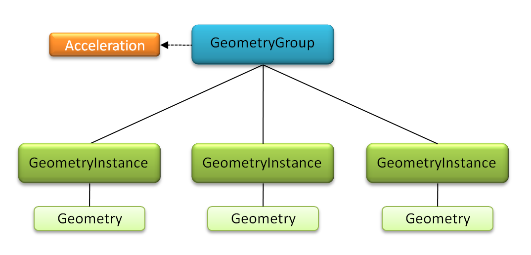
Figure 2 Multiple geometry instances in a geometry group
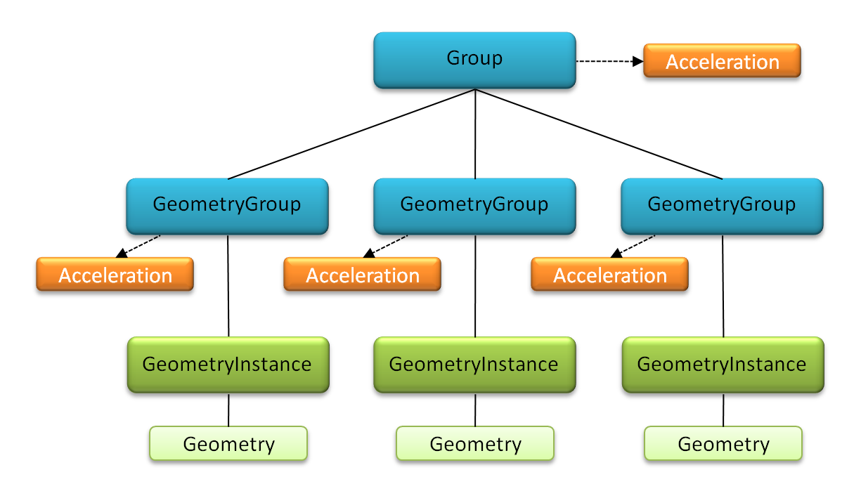
Figure 3 Multiple geometry instances, each in a separate geometry group
An rtAcceleration has a builder. The builder is responsible for collecting input geometry (in most cases, this geometry is the bounding boxes created by geometry nodes’ bounding box programs) and computing a data structure that allows for accelerated ray-scene intersection query. Builders are not application-defined programs. Instead, the application chooses an appropriate builder from Table 3:
| Builder | Description |
|---|---|
| Trbvh | The Trbvh3See Tero Karras and Timo Aila, Fast Parallel Construction of High-Quality Bounding Volume Hierarchies, http://highperformancegraphics.org/wp-content/uploads/Karras-BVH.pdf. builder performs a very fast GPU-based BVH build. Its ray tracing performance is usually within a few percent of SBVH, yet its build time is generally the fastest. This builder should be strongly considered for all datasets. Trbvh uses a modest amount of extra memory beyond that required for the final BVH. When the extra memory is not available on the GPU, Trbvh may automatically fallback to build on the CPU. |
| Sbvh | The Split-BVH (SBVH) is a high quality bounding volume hierarchy. While build times are highest, it was traditionally the method of choice for static geometry due to its high ray tracing performance, but may be superseded by Trbvh. Improvements over regular BVHs are especially visible if the geometry is non-uniform (e.g. triangles of different sizes). This builder can be used for any type of geometry, but for optimal performance with triangle geometry, specialized properties should be set (see Table 4)4See Martin Stich, Heiko Friedrich, Andreas Dietrich. Spatial Splits in Bounding Volume Hierarchies. http://www.nvidia.com/object/nvidia_research_pub_012.html.. |
| Bvh | The Bvh builder constructs a classic bounding volume hierarchy. It has
relatively good traversal performance and does not focus on fast
construction performance, but it supports refitting for fast incremental
updates (Table 4). Bvh is often the best choice for acceleration structures built over groups. |
| NoAccel | This is a dummy builder which does not construct an actual acceleration structure. Traversal loops over all elements and intersects each one with the ray. This is very inefficient for anything but very simple cases, but can sometimes outperform real acceleration structures, e.g. on a group with very few child nodes. |
Table 3 Supported builders
Table 3 shows the builders currently available in OptiX. A builder is set using rtAccelerationSetBuilder. The builder can be changed at any time; switching builders will cause an acceleration structure to be flagged for rebuild.
This example shows a typical initialization of an acceleration object:
RTacceleration accel;

rtAccelerationCreate( context, &accel );
rtAccelerationSetBuilder( accel, "Trbvh" );
Fine-tuning acceleration structure construction can be useful depending on the situation. For this purpose, builders expose various named properties, which are listed in Table 4:
| Property | Available in Builder | Description |
|---|---|---|
refit |
Bvh |
If set to 1, the builder will only readjust the node bounds of the bounding volume hierarchy instead of constructing it from scratch. Refit is only effective if there is an initial BVH already in place, and the underlying geometry has undergone relatively modest deformation. In this case, the builder delivers a very fast BVH update without sacrificing too much ray tracing performance. The default is 0. |
vertex_buffer_name |
Sbvh
|
The name of the buffer variable holding triangle vertex data. Each vertex consists of 3 floats. Mandatory for TriangleKdTree, optional for Sbvh (but recommended if the geometry consists of triangles). The default is vertex_buffer. |
vertex_buffer_stride |
Sbvh
|
The offset between two vertices in the vertex buffer, given in bytes. The default value is 0, which assumes the vertices are tightly packed. |
index_buffer_name |
Sbvh
|
The name of the buffer variable holding vertex index data. The entries in this buffer are indices of type int, where each index refers to one entry in the vertex buffer. A sequence of three indices represents one triangle. If no index buffer is given, the vertices in the vertex buffer are assumed to be a list of triangles, i.e. every 3 vertices in a row form a triangle.The default is index_buffer. |
index_buffer_stride |
Sbvh
|
The offset between two indices in the index buffer, given in bytes.
The default value is 0, which assumes the indices are tightly packed. |
chunk_size
|
Trbvh
|
Number of bytes to be used for a partitioned acceleration structure build. If no chunk size is set, or set to 0, the chunk size is chosen automatically. If set to -1, the chunk size is unlimited. The minimum chunk size is currently 64MB. Please note that specifying a small chunk size reduces the peak-memory footprint of the Trbvh, but can result in slower rendering performance. |
Table 4 Acceleration Structure Properties
Properties are specified using rtAccelerationSetProperty. Their values are given as strings, which are parsed by OptiX. Properties take effect only when an acceleration structure is actually rebuilt. Setting or changing the property does not itself mark the acceleration structure for rebuild; see the next section for details on how to do that. Properties not recognized by a builder will be silently ignored.
// Enable fast refitting on a BVH acceleration.
rtAccelerationSetProperty( accel, "refit", "1" );
In OptiX, acceleration structures are flagged (marked “dirty”) when they need to be rebuilt. During rtContextLaunch, all flagged acceleration structures are built before ray tracing begins. Every newly created rtAcceleration object is initially flagged dirty.
An application can decide at any time to explicitly mark an acceleration structure for rebuild. For example, if the underlying geometry of a geometry group changes, the acceleration structure attached to the geometry group must be recreated. This is achieved by calling rtAccelerationMarkDirty. This is also required if, for example, new child geometry instances are added to the geometry group, or if children are removed from it.
The same is true for acceleration structures on groups: adding or removing children, changing transforms below the group, etc., are operations which require the group’s acceleration to be marked as dirty. As a rule of thumb, every operation that causes a modification to the underlying geometry over which the structure is built (in the case of a group, that geometry is the children’s axis-aligned bounding boxes) requires a rebuild. However, no rebuild is required if, for example, some parts of the graph change further down the tree, without affecting the bounding boxes of the immediate children of the group.
Note that the application decides independently for each single acceleration structure in the graph whether a rebuild is necessary. OptiX will not attempt to automatically detect changes, and marking one acceleration structure as dirty will not propagate the dirty flag to any other acceleration structures. Failure to mark acceleration structures as dirty when necessary may result in unexpected behavior — usually missing intersections or performance degradation.
Mechanisms such as a graph node being attached as a child to multiple other graph nodes make composing the node graph flexible, and enable interesting instancing applications. Instancing can be seen as inexpensive reuse of scene objects or parts of the graph by referencing nodes multiple times instead of duplicating them.
OptiX decouples acceleration structures as separate objects from other graph nodes. Hence, acceleration structures can naturally be shared between several groups or geometry groups, as long as the underlying geometry on which the structure is built is the same:
// Attach one acceleration to multiple groups.
rtGroupSetAcceleration( group1, accel );
rtGroupSetAcceleration( group2, accel );
rtGroupSetAcceleration( group3, accel );
Note that the application must ensure that each node sharing the acceleration structure has matching underlying geometry. Failure to do so will result in undefined behavior. Also, acceleration structures cannot be shared between groups and geometry groups.
The capability of sharing acceleration structures is a powerful concept to maximize efficiency, as shown in Figure 4. The acceleration node in the center of the figure is attached to both geometry groups, and both geometry groups reference the same geometry objects. This reuse of geometry and acceleration structure data minimizes both memory footprint and acceleration construction time. Additional geometry groups could be added in the same manner at very little overhead.
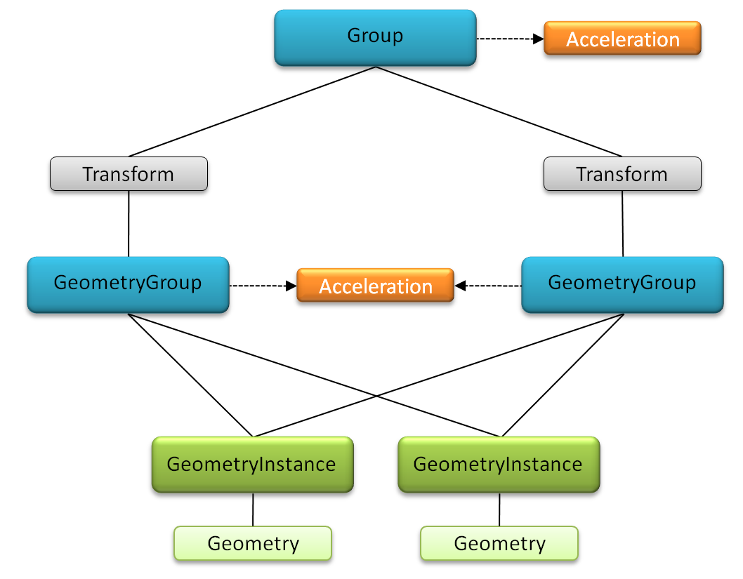
Figure 4 Two geometry groups sharing an acceleration structure and the underlying geometry objects.
OptiX 3.8 introduced remote network rendering as well as a new type of launch called the progressive launch. Using these APIs, common progressive rendering algorithms can be implemented easily and executed efficiently on NVIDIA’s Visual Computing Applicance servers (VCAs). All OptiX computation can happen remotely on the VCA, with the rendered result being sent back to the client as a video stream. This allows even relatively low-performance client computers to run heavyweight OptiX applications efficiently, using the substantial computational resources provided by tens or hundreds of GPUs in a VCA cluster.
The Progressive Launch API mainly serves to address the following aspects not covered by the traditional OptiX API:
The rtContextLaunch calls offered by traditional OptiX work for remote rendering but are not well suited to it. Because the API calls are synchronous, each launch/display cycle incurs the full network roundtrip latency, and thus performance is usually not acceptable over standard network connections. Progressive launches, on the other hand, are asynchronous, and can achieve smooth application performance even over a high latency connection.
OptiX can parallelize work across a small number of local GPUs. To enable first class support for VCA clusters, however, the system needs to be able to scale to potentially hundreds of GPUs efficiently. Progressive renderers, such as path tracers, are one of the most common use cases of OptiX. The fact that the image samples they compute are independent of each other provides a natural way to parallelize the problem. The Progressive Launch API therefore combines the assumption that work can be split into many independent parts with the capability to launch kernels asynchronously.
Note that the Progressive Launch API may be used to render on local devices, as well as remotely on the VCA. Except for the code that sets up the RemoteDevice (see Remote Devices), whether rendering happens locally or remotely is transparent to the application. For applications that are amenable to the progressive launch programming model an advantage of using this model all the time, rather than traditional synchronous launches is that adapting the application to the VCA with full performance is virtually automatic.
The connection to a VCA (or cluster of VCAs) is represented by the Rtremotedevice API object. On creation, the network connection is established given the URL of the cluster manager (in form of a WebSockets address) and user credentials. Information about the device can then be queried using rtRemoteDeviceGetAttribute. A VCA cluster consists of a number of nodes, of which a subset can be reserved for rendering using rtRemoteDeviceReserve. Since several server configurations may be available, that call also selects which one to use.
After node reservation has been initiated, the application must wait for the nodes to be ready by polling the RT_REMOTEDEVICE_STATUS attribute. Once that flag reports RT_REMOTEDEVICE_STATUS_READY, the device can be used for rendering.
To execute OptiX commands on the remote device, the device must be assigned to a context using rtContextSetRemoteDevice. Note that only newly created contexts can be used with remote devices. That is, the call to rtContextSetRemoteDevice should immediately follow the call to rtContextCreate.
While most existing OptiX applications will work unchanged when run on a remote device (see Limitations for caveats), progressive launches must be used instead of rtContextLaunch for optimal performance.
Instead of requesting the generation of a single frame, a progressive launch, triggered by rtContextLaunchProgressive2D, requests multiple subframes at once. A subframe is output buffer content which is composited with other subframes to yield the final frame. In most progressive renderers, this means that a subframe simply contains a single sample per pixel.
Progressive launch calls are non-blocking. An application typically executes a progressive launch, and then continuously polls the stream buffers associated with its output, using rtBufferGetProgressiveUpdateReady. If that call reports that an update is available, the stream buffer can be mapped and the content displayed.
If any OptiX API functions are called while a progressive launch is in progress, the launch will stop generating subframes until the next time a progressive launch is triggered (the exception is the API calls to poll and map the stream buffers). This way, state changes to OptiX, such as setting variables using rtVariableSet, can be made easily and efficiently in combination with a render loop that polls for stream updates and executes a progressive launch. This method is outlined in the example pseudocode below.
Accessing the results of a progressive launch is typically done through a new type of buffer called a stream buffer. Stream buffers allow the remotely rendered frames to be sent to the application client using compressed video streaming, greatly improving response times while still allowing the application to use the result frame in the same way as with a non-stream output buffer.
Stream buffers are created using rtBufferCreate with the type set to RT_BUFFER_PROGRESSIVE_STREAM. A stream buffer must be bound to a regular output buffer via rtBufferBindProgressiveStream in order to define its data source.
By executing the bind operation, the system enables automatic compositing for the output buffer. That is, any values written to the output buffer by device code will be averaged into the stream buffer, rather than overwriting the previous value as in regular output buffers. Compositing happens automatically and potentially in parallel across many devices on the network, or locally if remote rendering is not used.
Several configuration options are available for stream buffers, such as the video stream format to use, and parameters to trade off quality versus speed. Those options can be set using rtBufferSetAttribute. Note that some of the options only take effect if rendering happens on a remote device, and are a no-op when rendering locally. This is because stream buffers don’t undergo video compression when they don’t have to be sent across a network.
In addition to automatic compositing, the system also tonemaps and quantizes the averaged output before writing it into a stream. Tonemapping is performed using a simple built-in operator with a user-defined gamma value (specified using rtBufferSetAttribute). The tonemap operator is defined as:
final_value = clamp( pow( hdr_value, 1/gamma ), 0, 1 )
Accessing a progressive stream happens by mapping the stream buffer, just like any regular buffer, and reading out the frame data. The data is uncompressed, if necessary, when mapped. The data available for reading will always represent the most recent update to the stream if a progressive launch is in progress, so a frame that is not read on time may be skipped (e.g., if polling happens at a low frequency).
It is also possible to map an output buffer that is bound as a data source for a stream buffer. This can be useful to access “final frame” data, i.e. the uncompressed and unquantized accumulated output. Note that mapping a non-stream buffer will cause the progressive launch to stop generating subframes, and that such a map operation is much slower than mapping a stream.
In OptiX device code, the subframe index used for progressive rendering is exposed as a semantic variable of type unsigned int. Its value is guaranteed to be unique for each subframe in the current progressive launch, starting at zero for the first subframe and increasing by one with each subsequent subframe. For example, an application performing stochastic sampling may use this variable to seed a random number generator.
The current subframe index can be accessed in shader programs by declaring the following variable:
rtDeclareVariable(unsigned int, index, rtSubframeIndex,);
Computed pixel values can be written to an output buffer, just like for non-progressive rendering. Output buffers that are bound as sources to stream buffers will then be averaged automatically and processed as described in the section on Buffers.
Note in particular that device code does not use stream buffers directly.
RT_BUFFER_INPUT_OUTPUT in combination with remote rendering yields undefined results.rtPrintf and associated host functions are not supported in combination with remote rendering.rtContextSetTimeoutCallback is not supported in combination with remote rendering.RT_FORMAT_FLOAT3 or RT_FORMAT_FLOAT4 format. For performance reasons, using RT_FORMAT_FLOAT4 is strongly recommended.RT_FORMAT_UNSIGNED_BYTE4 format.For complete example applications using remote rendering and progressive launches, please refer to the "progressive" and "queryRemote" samples in the SDK. The following illustrates basic API usage in pseudocode.
// Set up the remote device. To use progressive rendering locally,
// simply skip this and the call to rtContextSetRemoteDevice.
RTremotedevice rdev;
rtRemoteDeviceCreate( "wss://myvcacluster.example.com:443",
     "user", "password", &rdev );

// Reserve 1 VCA node with config #0
rtRemoteDeviceReserve( rdev, 1, 0 );

// Wait until the VCA is ready
int ready;
bool first = true;

do {
     if (first)
         first = false;
     else
         sleep(1); // poll once per second.

     rtRemoteDeviceGetAttribute( rdev,
          RT_REMOTEDEVICE_ATTRIBUTE_STATUS,
          sizeof(int), &ready ) );
} while( ready != RT_REMOTEDEVICE_STATUS_READY );

// Set up the Optix context
RTcontext context;
rtContextCreate( &context );

// Enable rendering on the remote device. Must immediately
// follow context creation.
rtContextSetRemoteDevice( context, rdev );

// Set up a stream buffer/output buffer pair
RTbuffer output_buffer, stream_buffer;
rtBufferCreate( context, RT_BUFFER_OUTPUT, &output_buffer );
rtBufferCreate( context, RT_BUFFER_PROGRESSIVE_STREAM,
     &stream_buffer );

rtBufferSetSize2D( output_buffer, width, height );
rtBufferSetSize2D( stream_buffer, width, height );
rtBufferSetFormat( output_buffer, RT_FORMAT_FLOAT4 );
rtBufferSetFormat( stream_buffer, RT_FORMAT_UNSIGNED_BYTE4 );

rtBufferBindProgressiveStream( stream_buffer, output_buffer );

// [The usual OptiX scene setup goes here. Geometries, acceleration
// structures, materials, programs, etc.]

// Non-blocking launch, request infinite number of subframes
rtContextLaunchProgressive2D( context, width, height, 0 );

while( !finished )
{
     // Poll stream buffer for updates from the progressive launch
     int ready;
     rtBufferGetProgressiveUpdateReady( stream_buffer, &ready, 0, 0 );

     if( ready )
     {
          // Map and display the stream. This won't interrupt rendering.
          rtBufferMap( stream_buffer, &data );
          display( data );
          rtBufferUnmap( stream_buffer );
     }

     // Check whether scene has changed, e.g. because of user input
     if( scene_changed() )
     {
          // [Update OptiX state here, e.g. by calling rtVariableSet
          // or other OptiX functions. This will cause the server to
          // stop generating subframes, so we call launch again below].
          rtVariableSet( ... );
     }

     // Start a new progressive launch, in case the OptiX state has been
     // changed above. If it hasn't, then this is a no-op and the
     // previous launch just continues running, accumulating further
     // subframes into the stream.
     rtContextLaunchProgressive2D( context, width, height, 0 );
}

// Clean up.
rtContextDestroy( context );
rtRemoteDeviceRelease( rdev );
rtRemoteDeviceDestroy( rdev );

NVIDIA® GameWorks™ Documentation Rev. 1.0.171006 ©2014-2017. NVIDIA Corporation. All Rights Reserved.