Using AIPerf to Benchmark#

NVIDIA AIPerf is a client-side generative AI benchmarking tool that reports TTFT, ITL, TPS, RPS, and related metrics. It works with any OpenAI-compatible inference service, including NVIDIA NIM. This section walks through benchmarking a Llama-3 model with AIPerf.

For metric definitions, refer to Metrics. For parameter guidance, refer to Parameters and Best Practices.

Set Up an OpenAI-Compatible Llama-3 Inference Service with NVIDIA NIM#

NVIDIA NIM provides the easiest and quickest way to put an LLM into production. Refer to the NIM LLM getting started documentation for comprehensive guidance.

During startup, the NIM container downloads the required resources and begins serving the model behind an API endpoint. The following message indicates a successful startup:

(APIServer pid=74) INFO:     Started server process [74]
(APIServer pid=74) INFO:     Waiting for application startup.
(APIServer pid=74) INFO:     Application startup complete.

After startup, NIM provides an OpenAI-compatible API that you can query, as shown in the following example:

# Run `pip install openai` before running this Python code

from openai import OpenAI
client = OpenAI(base_url="http://0.0.0.0:8000/v1", api_key="not-used")
prompt = "Once upon a time"
response = client.completions.create(
    model="meta/llama-3.1-8b-instruct",
    prompt=prompt,
    max_tokens=16,
    stream=False
)
completion = response.choices[0].text
print(completion)

Note

NVIDIA benchmarking tests show that additional Docker flags can improve inference performance. Use either --security-opt seccomp=unconfined, which disables the Seccomp security profile, or --privileged, which grants the container broad host capabilities, including direct access to hardware, device files, and some kernel functionality. These flags improved performance by up to 5% with the NIM TensorRT-LLM v0.10.0 backend and up to 20% with the OSS vLLM backend tested on v0.4.3 or the NIM vLLM backend tested on NIM 1.0.0. NVIDIA verified this behavior on DGX A100 and H100 systems. These flags can reduce container security overhead, but they also elevate security risk. Use them only after reviewing your security requirements. Refer to the Docker privileged container documentation for more information.

Set Up AIPerf and Warm Up: Benchmarking a Single Use Case#

After the NIM Llama-3 inference service is running, set up AIPerf. The easiest approach is a pre-built Docker container. Run AIPerf on the same host as NIM to avoid network latency, unless you intentionally want to include network effects in the measurement.

Note

Refer to the AIPerf documentation for comprehensive setup guidance.

Run the following commands to use the NVIDIA Triton Server pre-built container.

export RELEASE="26.06" # recommend using latest releases in yy.mm format
export WORKDIR=<YOUR_AI_PERF_WORKING_DIRECTORY>

docker run -it --net=host --gpus=all -v $WORKDIR:/workdir nvcr.io/nvidia/tritonserver:${RELEASE}-py3-sdk

After you start the container, install AIPerf:

pip install aiperf

Note

This test uses the llama-3 tokenizer from Hugging Face, which is a guarded Meta-Llama-3.1-8B-Instruct repository. You need to apply for access, then log in with your Hugging Face credential.

pip install huggingface_hub
hf auth login

Then, start the AIPerf evaluation harness, which runs a warm-up load test on the NIM backend:

export INPUT_SEQUENCE_LENGTH=200
export INPUT_SEQUENCE_STD=10
export OUTPUT_SEQUENCE_LENGTH=200
export CONCURRENCY=10
export REQUEST_COUNT=$(($CONCURRENCY * 3))
export MODEL=meta/llama-3.1-8b-instruct

cd /workdir
aiperf profile \
   -m $MODEL \
   --endpoint-type chat \
   --streaming \
   -u localhost:8000 \
   --synthetic-input-tokens-mean $INPUT_SEQUENCE_LENGTH \
   --synthetic-input-tokens-stddev $INPUT_SEQUENCE_STD \
   --concurrency $CONCURRENCY \
   --request-count $REQUEST_COUNT \
   --output-tokens-mean $OUTPUT_SEQUENCE_LENGTH \
   --extra-inputs min_tokens:$OUTPUT_SEQUENCE_LENGTH \
   --extra-inputs ignore_eos:true \
   --tokenizer meta-llama/llama-3.1-8b-instruct \
   --profile-export-file ${INPUT_SEQUENCE_LENGTH}_${OUTPUT_SEQUENCE_LENGTH}.json

This example specifies the input sequence length, output sequence length, and concurrency to test. It also tells the backend to ignore the EOS token so the output reaches the intended length.

Note

Refer to the AIPerf CLI options documentation for the full set of options and parameters.

After successful execution, results similar to the following appear in the terminal:
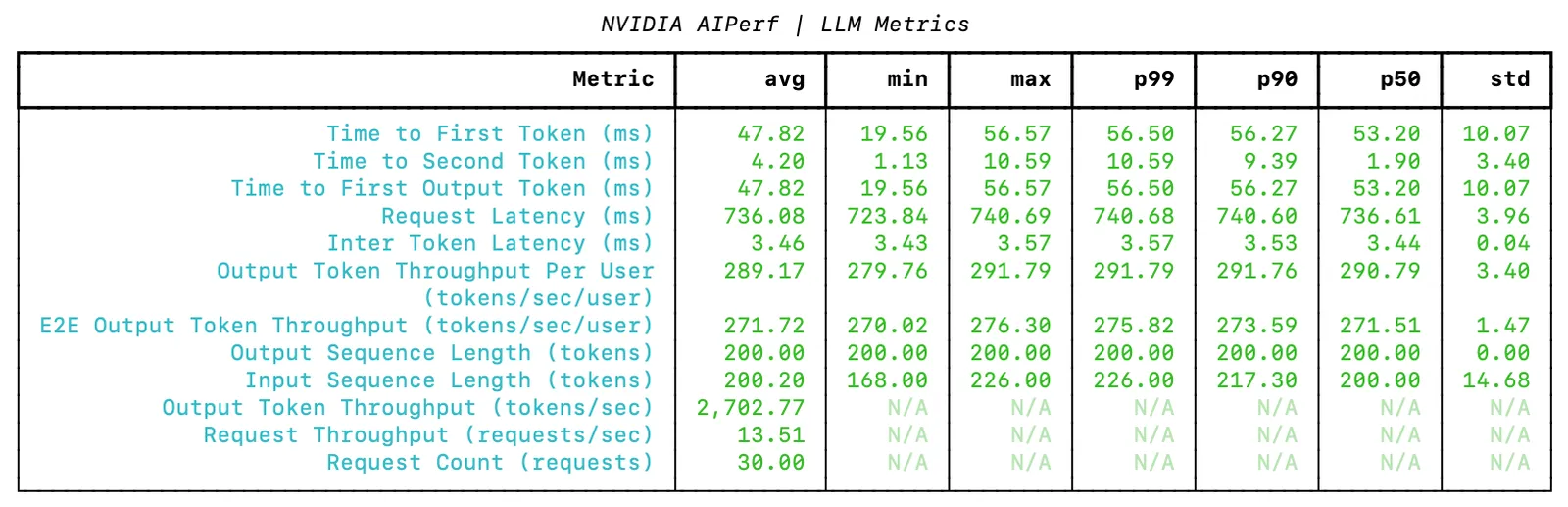
_images/image6.png

Figure 6. Sample output by AIPerf.#

Sweep through a Number of Use Cases#

Benchmarking usually sweeps across use cases, such as input/output length combinations, and load scenarios, such as different concurrency values. Use the following Bash script to define the parameters so AIPerf runs all combinations.

Note

Before running a full sweep, run a warm-up test as shown in the previous section.

declare -A useCases

# Populate the array with use case descriptions and their specified input/output lengths
useCases["Translation"]="200/200"
useCases["Text classification"]="200/5"
useCases["Text summary"]="1000/200"

# Function to execute AIPerf with the input/output lengths as arguments
runBenchmark() {
   local description="$1"
   local lengths="${useCases[$description]}"
   IFS='/' read -r inputLength outputLength <<< "$lengths"

   echo "Running AIPerf for $description with input length $inputLength and output length $outputLength"
   #Runs
   for concurrency in 1 2 5 10 50 100 250; do

       local INPUT_SEQUENCE_LENGTH=$inputLength
       local INPUT_SEQUENCE_STD=0
       local OUTPUT_SEQUENCE_LENGTH=$outputLength
       local CONCURRENCY=$concurrency
       local REQUEST_COUNT=$(($CONCURRENCY * 3))
       local MODEL=meta/llama-3.1-8b-instruct

       aiperf profile \
           -m $MODEL \
           --endpoint-type chat \
           --streaming \
           -u localhost:8000 \
           --synthetic-input-tokens-mean $INPUT_SEQUENCE_LENGTH \
           --synthetic-input-tokens-stddev $INPUT_SEQUENCE_STD \
           --concurrency $CONCURRENCY \
           --request-count $REQUEST_COUNT \
           --output-tokens-mean $OUTPUT_SEQUENCE_LENGTH \
           --extra-inputs min_tokens:$OUTPUT_SEQUENCE_LENGTH \
           --extra-inputs ignore_eos:true \
           --tokenizer meta-llama/llama-3.1-8b-instruct \
           --artifact-dir artifact/ISL${INPUT_SEQUENCE_LENGTH}_OSL${OUTPUT_SEQUENCE_LENGTH}/CON${CONCURRENCY}

   done
}

# Iterate over all defined use cases and run the benchmark script for each
for description in "${!useCases[@]}"; do
   runBenchmark "$description"
done

Save this script in a working directory, such as /workdir/benchmark.sh. Run it with the following command:

cd /workdir
bash benchmark.sh

Note

The --request-count parameter specifies the number of requests for the measurement. This example sets it to three times the concurrency level to obtain a stable measurement. High concurrency on a large model with a large ISL/OSL scenario can significantly increase benchmark time.

Analyze the Output#

When the tests complete, AIPerf writes structured outputs under an artifact directory in your mounted working directory (/workdir in these examples), organized by input/output length and concurrency. Your results should resemble the following.

/workdir/artifact
 └── ISL200_OSL200
     ├── CON1
     |   ├── logs
     |   |   └── aiperf.log
     |   ├── profile_export_aiperf.csv
     |   └── profile_export_aiperf.json
     ├── CON10
     |   ├── logs
     |   |   └── aiperf.log
     |   ├── profile_export_aiperf.csv
     |   └── profile_export_aiperf.json
     ├── CON100
     |   ├── logs
     |   |   └── aiperf.log
     |   ├── profile_export_aiperf.csv
     |   └── profile_export_aiperf.json
     ├── CON2
     |   ├── logs
     |   |   └── aiperf.log
     |   ├── profile_export_aiperf.csv
     |   └── profile_export_aiperf.json
...

The profile_export_aiperf.json files contain the main benchmarking results. Use the following Python snippet to load a result file for one use case:

import json

with open('artifact/ISL200_OSL5/CON1/profile_export_aiperf.json', 'r') as f:
    data = json.load(f)

You can also collect tokens-per-second and TTFT metrics across concurrencies for a given use case:

import os

ISL = 200
OSL = 5

concurrencies = [1, 2, 5, 10, 50, 100, 250]
TPS = []
TTFT = []

for con in concurrencies:
   with open(f'artifact/ISL{ISL}_OSL{OSL}/CON{con}/profile_export_aiperf.json', 'r') as f:
       data = json.load(f)
       TPS.append(data['output_token_throughput']['avg'])
       TTFT.append(data['time_to_first_token']['avg'])

Finally, plot and analyze the latency-throughput curve with the collected data. Each point corresponds to a concurrency value.

import matplotlib.pyplot as plt

# Assuming TTFT, TPS, and concurrencies are defined lists or arrays
# (e.g., TTFT = [0.5, 1.2, 2.0], TPS = [100, 80, 50], concurrencies = [1, 2, 4])

# Create the figure and axes
plt.figure()

# Plot the line
plt.plot(TTFT, TPS, marker='o') # 'marker' helps see the points

# Add the text labels (equivalent to 'text=concurrencies')
if 'concurrencies' in locals() and concurrencies is not None:
    for i in range(len(TTFT)):
        plt.text(TTFT[i], TPS[i], str(concurrencies[i]),
                 ha='center', va='bottom', fontsize=9) # Adjust ha/va/fontsize as needed

# Set axis labels (equivalent to update_layout)
plt.xlabel("Single User: time to first token(s)")
plt.ylabel("Total System: tokens/s")

# Add a grid (Plotly usually has one by default)
plt.grid(True)

# Display the plot (equivalent to fig.show())
plt.show()

The resulting plot from AIPerf measurement data looks like the following:
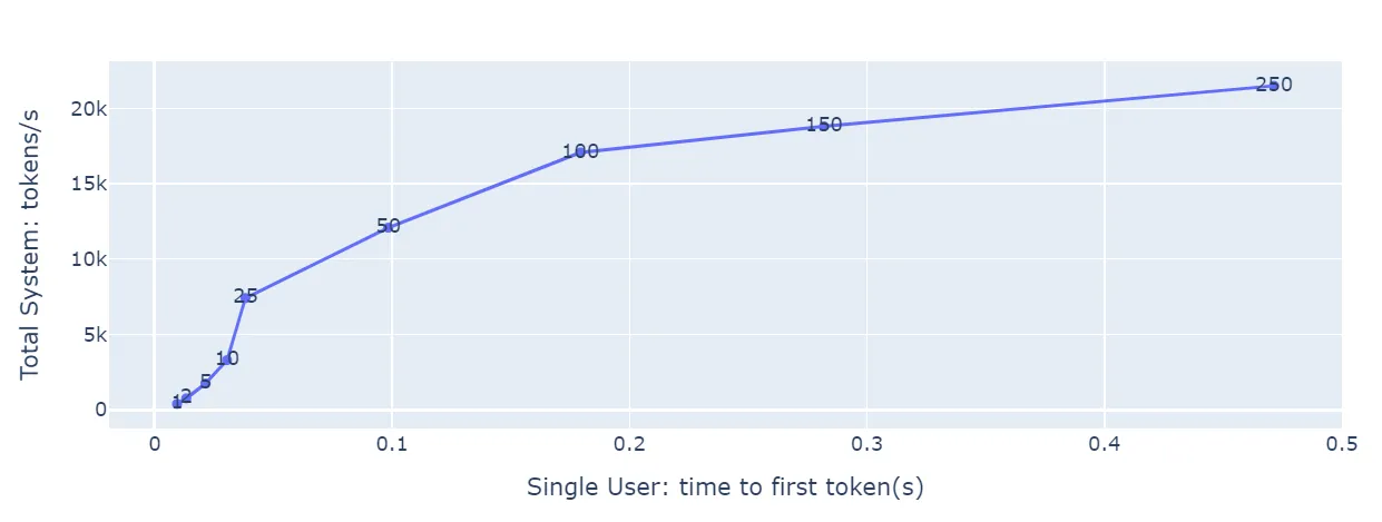
_images/image5.png

Figure 7: Latency-throughput curve plot using data generated by AIPerf.#

Interpret the Results#

The previous plot shows TTFT on the x-axis, total system throughput on the y-axis, and concurrencies on each dot. You can use the plot in two ways:

  1. If you have a latency budget, use the maximum acceptable TTFT as the x value. The matching y value and concurrency show the highest throughput you can achieve within that latency limit.

  2. If you have a target concurrency, locate that dot on the graph. The matching x and y values show latency and throughput for that concurrency level.

The plot also shows concurrencies where latency grows quickly with little or no throughput gain. For example, in the plot above, concurrency=100 is one such value.

Similar plots can use ITL, e2e_latency, or TPS_per_user as the x-axis to show the trade-off between total system throughput and individual latency.