Quickstart Guide for NVIDIA Earth-2 Correction Diffusion NIM#
Use this documentation to get started with NVIDIA Earth-2 Correction Diffusion (CorrDiff) NIM.
Important
Before you can use this documentation, you must satisfy all prerequisites.
Warning
This quick start guide is designed for use with Nvidia’s A100 or H100 GPUs.
GPUs with lower VRAM and/or compute may require EARTH2NIM_TARGET_BATCHSIZE to be lowered or the time out in the post request to be increased.
See the configuration page for different deployment options.
Workflow Overview#
This guide walks you through the complete CorrDiff NIM workflow, from deployment to generating downscaled weather predictions. The end-to-end process consists of four main stages:
Deployment: Pull and launch the CorrDiff NIM container, which hosts the pre-trained model and provides an HTTP API for inference.
Data Preparation: Fetch and preprocess input weather data from public sources. The default model expects GEFS (Global Ensemble Forecast System) data at 0.25-degree resolution (~25km) over the contiguous United States. This guide uses Earth2Studio to simplify data fetching and formatting.
Inference: Send your prepared input data to the NIM’s API endpoint. The diffusion model generates multiple high-resolution samples (3km resolution) by correcting and downscaling the input data. You can control the generation process through parameters like sample count, diffusion steps, and random seed.
Output Processing: Retrieve and visualize the results. The NIM returns downscaled weather fields in NumPy array format packaged as a tar archive. Each sample represents a plausible high-resolution forecast that captures uncertainty and extreme events better than traditional deterministic methods.
The sections below guide you through each stage with practical examples using both Bash and Python.
Launching the NIM#
Pull the NIM container with the following command.
Note
The container is ~26GB (uncompressed) and the download time depends on internet connection speeds.
docker pull nvcr.io/nim/nvidia/corrdiff:1.1.0
Run the NIM container with the following command. This command starts the NIM container and exposes port 8000 for the user to interact with the NIM. It pulls the model on the local filesystem.
Note
The model is ~4GB and the download time depends on internet connection speeds.
export NGC_API_KEY=<NGC API Key>

docker run --rm --runtime=nvidia --gpus all --shm-size 4g \
    -p 8000:8000 \
    -e NGC_API_KEY \
    -t nvcr.io/nim/nvidia/corrdiff:1.1.0
After the NIM is running, you see output similar to the following:
I0829 05:18:42.152983 108 grpc_server.cc:2466] "Started GRPCInferenceService at 0.0.0.0:8001"
I0829 05:18:42.153277 108 http_server.cc:4638] "Started HTTPService at 0.0.0.0:8090"
I0829 05:18:42.222628 108 http_server.cc:320] "Started Metrics Service at 0.0.0.0:8002"
Checking NIM Health#
Open a new terminal, leaving the current terminal open with the launched service.
Wait until the health check end point returns
{"status":"ready"}before proceeding. This might take a couple of minutes. Use the following methods to query the health check.
Bash#
curl -X 'GET' \
    'http://localhost:8000/v1/health/ready' \
    -H 'accept: application/json'
Python#
import requests

r = requests.get("http://localhost:8000/v1/health/ready")
if r.status_code == 200:
   print("NIM is healthy!")
else:
   print("NIM is not ready!")
Fetching Input Data#
The CorrDiff NIM launches with a default model profile trained for downscaling over the contiguous United States. The input to this model is GEFS weather data at 0.25-degree (~25km) resolution over the United States, sourced from NOAA. CorrDiff use this input data to generate downscaled weather fields at a 3km resolution, similar to NOAA’s HRRR model. For additional details, refer to the model card.
To simplify data preparation, we use Earth2Studio to fetch and format the input data as follows:
Fetch a set of select GEFS variable at a resolution 0.25-degrees on a lat-lon grid.
Fetch a set of regular GEFS variables at a resolution of 0.5-degrees and interpolate to 0.25 degree grid on a lat-lon grid.
Crop both variables to a bounded box over the United States.
Concatenate both sets of variables as well as an integer field that denotes the forecast lead time the input represents.
Use the script below to download and structure the data:
from datetime import datetime, timedelta

import numpy as np
import torch
from earth2studio.data import GEFS_FX, HRRR, GEFS_FX_721x1440

GEFS_SELECT_VARIABLES = [
    "u10m",
    "v10m",
    "t2m",
    "r2m",
    "sp",
    "msl",
    "tcwv",
]

GEFS_VARIABLES = [
    "u1000",
    "u925",
    "u850",
    "u700",
    "u500",
    "u250",
    "v1000",
    "v925",
    "v850",
    "v700",
    "v500",
    "v250",
    "z1000",
    "z925",
    "z850",
    "z700",
    "z500",
    "z200",
    "t1000",
    "t925",
    "t850",
    "t700",
    "t500",
    "t100",
    "r1000",
    "r925",
    "r850",
    "r700",
    "r500",
    "r100",
]

ds_gefs = GEFS_FX(cache=True)
ds_gefs_select = GEFS_FX_721x1440(cache=True, member="gec00")


def fetch_input_gefs(
    time: datetime, lead_time: timedelta, content_dtype: str = "float32"
):
    """Fetch input GEFS data and place into a single numpy array

    Parameters
    ----------
    time : datetime
        Time stamp to fetch
    lead_time : timedelta
        Lead time to fetch
    filename : str
        File name to save input array to
    content_dtype : str
        Numpy dtype to save numpy
    """
    dtype = np.dtype(getattr(np, content_dtype))
    # Fetch high-res select GEFS input data
    select_data = ds_gefs_select(time, lead_time, GEFS_SELECT_VARIABLES)
    select_data = select_data.values
    # Crop to bounding box [225, 21, 300, 53]
    select_data = select_data[:, 0, :, 148:277, 900:1201].astype(dtype)
    assert select_data.shape == (1, len(GEFS_SELECT_VARIABLES), 129, 301)

    # Fetch GEFS input data
    pressure_data = ds_gefs(time, lead_time, GEFS_VARIABLES)
    # Interpolate to 0.25 grid
    pressure_data = torch.nn.functional.interpolate(
        torch.Tensor(pressure_data.values),
        (len(GEFS_VARIABLES), 721, 1440),
        mode="nearest",
    )
    pressure_data = pressure_data.numpy()
    # Crop to bounding box [225, 21, 300, 53]
    pressure_data = pressure_data[:, 0, :, 148:277, 900:1201].astype(dtype)
    assert pressure_data.shape == (1, len(GEFS_VARIABLES), 129, 301)

    # Create lead time field
    lead_hour = int(lead_time.total_seconds() // (3 * 60 * 60)) * np.ones(
        (1, 1, 129, 301)
    ).astype(dtype)

    input_data = np.concatenate([select_data, pressure_data, lead_hour], axis=1)[None]
    return input_data


input_array = fetch_input_gefs(datetime(2023, 1, 1), timedelta(hours=0))
np.save("corrdiff_inputs.npy", input_array)
Running the script will generate the NumPy array corrdiff_inputs.npy, which is now ready to use with the model.
Inference Request#
With the pre-processed input for this CorrDiff US model, the API to the NIM can now be used as follows. The NumPy array is sent to the NIM as a file along with several other parameters that can be used to control the underlying diffusion model. For complete documentation on the API specification of the NIM, visit the API documentation page.
Bash#
curl -X POST \
    -F "input_array=@corrdiff_inputs.npy" \
    -F "samples=2" \
    -F "steps=12" \
    -o output.tar \
    http://localhost:8000/v1/infer
Python#
import requests

url = "http://localhost:8000/v1/infer"
files = {
    "input_array": ("input_array", open("corrdiff_inputs.npy", "rb")),
}
data = {
    "samples": 2,
    "steps": 14,
    "seed": 0,
}
headers = {
    "accept": "application/x-tar",
}
print("Sending post request to NIM")

# Adjust time out (seconds) below
r = requests.post(url, headers=headers, data=data, files=files, timeout=180)

if r.status_code != 200:
    raise Exception(r.content)
else:
    # Dump response to file
    with open("output.tar", "wb") as tar:
        tar.write(r.content)
Results#
The results are inside a tar file that can be explored using:
tar -tvf output.tar

-rw-r--r-- 0/0        60555392 1970-01-01 00:00 000_000.npy
-rw-r--r-- 0/0        60555392 1970-01-01 00:00 001_000.npy
Tip
The tar archive is populated with NumPy arrays that have the naming convention {sample index}_{batch index}.npy.
Important
For most inference calls, it is important to specify a longer timeout period for a request to this NIM. Refer to the performance data for estimated inference speeds on different GPU models.
Streaming Responses#
The CorrDiff NIM can be used to stream back samples as they are generated in instances where the client requests a larger sample size than the NIMs inference batch size. This can be extremely useful when creating a pipeline that runs following processes on each time-step. The follow snippet can be used to access each time-step, in memory, from the NIM as it is generated.
Note
The environment variable EARTH2NIM_TARGET_BATCHSIZE governs the batch size used inside the NIM. When this value is lower than the requested sample size, streaming the results back can be useful. See the configuration guide for more details on this parameter.
import io
import tarfile
from pathlib import Path

import numpy as np
import requests
import tqdm

url = f"http://localhost:8000/v1/infer"
files = {
    "input_array": ("input_array", open("corrdiff_inputs.npy", "rb")),
}
data = {
    "samples": 16,
    "steps": 8,
    "seed": 0,
}
headers = {
    "accept": "application/x-tar",
}

pbar = tqdm.tqdm(range(data["samples"]), desc="CorrDiff samples")
with (
    requests.post(
        url,
        headers=headers,
        files=files,
        data=data,
        timeout=300,
        stream=True,
    )
) as resp:
    resp.raise_for_status()
    with tarfile.open(fileobj=resp.raw, mode="r|") as tar_stream:
        # Loop over file members from tar stream
        for member in tar_stream:
            arr_file = io.BytesIO()
            arr_file.write(tar_stream.extractfile(member).read())
            arr_file.seek(0)
            data = np.load(arr_file)
            # Array names are in the form <BATCH_IDX>_<SAMPLE_IDX>.npy
            arr_sample_idx, _ = (
                int(x) for x in Path(member.name).stem.split("_", maxsplit=1)
            )

            pbar.write(f"Received data for sample {arr_sample_idx}")
            pbar.write(f"Output numpy {member.name} with shape {data.shape}")
            pbar.update(1)
Post Processing#
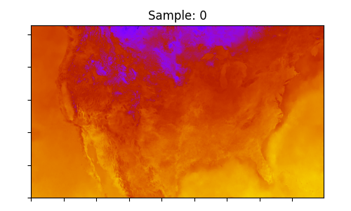
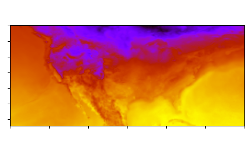
The final step is to perform some basic visualization of the results. The surface temperature is plotted from both the input and output arrays.
Note
The CorrDiff NIM returns the raw output data array. Additional metadata must be processed client side using information in the model card. The latitude and longitude coordinate values can be obtained from the corrdiff_output_lat.npy and corrdiff_output_lon.npy files in the model package.
import matplotlib.pyplot as plt
import numpy as np
import tarfile
import io
# Output variables: [u10m, v10m, t2m, tp, csnow, cicep, cfrzr, crain]
variable = 2
input = np.load("corrdiff_inputs.npy")
fig, ax = plt.subplots(1,1, figsize=(5,3))
ax.imshow(input[0,0,variable], cmap="gnuplot")
ax.set_yticklabels([])
ax.set_xticklabels([])
fig.tight_layout()
plt.savefig("input_t2m.png")
with tarfile.open("output.tar") as tar:
for i, member in enumerate(tar.getmembers()):
arr_file = io.BytesIO()
arr_file.write(tar.extractfile(member).read())
arr_file.seek(0)
data = np.load(arr_file)
plt.close("all")
fig, ax = plt.subplots(1,1, figsize=(5,3))
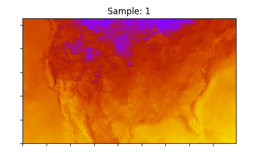
ax.set_title(f"Sample: {i}")
ax.imshow(data[0,0,variable], origin='lower', cmap="gnuplot")
ax.set_yticklabels([])
ax.set_xticklabels([])
fig.tight_layout()
plt.savefig(f"output_t2m_sample_{i}.png")
Input surface temperature contour at ~25km resolution:
Output surface temperature samples downscaled using CorrDiff to 3km resolution: