Quickstart Guide for DoMINO-Automotive-Aero NIM#
Use this documentation to get started with DoMINO-Automotive-Aero NIM.
Important
Before you can use this documentation, you must satisfy all prerequisites.
Launching the NIM#
Pull the NIM container with the following command.
Note
The container is ~31GB (uncompressed) and the download time depends on internet connection speeds.
docker pull nvcr.io/nim/nvidia/domino-automotive-aero:2.1.0-41313772
Run the NIM container with the following command. This command starts the NIM container and exposes port 8000 for the user to interact with the NIM. It pulls the model on the local filesystem.
Note
The model is ~91MB and the download time depends on internet connection speeds.
export NGC_API_KEY=<NGC API Key>

docker run --rm --runtime=nvidia --gpus 1 --shm-size 2g \
    -p 8000:8000 \
    -e NGC_API_KEY \
    -t nvcr.io/nim/nvidia/domino-automotive-aero:2.1.0-41313772
After the NIM is running, you see output similar to the following:
I0212 23:07:14.639570 253 grpc_server.cc:2463] "Started GRPCInferenceService at 0.0.0.0:8001"
I0212 23:07:14.640137 253 http_server.cc:4695] "Started HTTPService at 0.0.0.0:8080"
I0212 23:07:14.743047 253 http_server.cc:358] "Started Metrics Service at 0.0.0.0:8002"
Checking NIM Health#
Open a new terminal, leaving the current terminal open with the launched service.
Wait until the health check end point returns
{"status":"ready"}before proceeding. This might take a couple of minutes. Use the following methods to query the health check.
Bash#
curl -X 'GET' \
    'http://localhost:8000/v1/health/ready' \
    -H 'accept: application/json'
Python#
import httpx

r = httpx.get("http://localhost:8000/v1/health/ready")
if r.status_code == 200:
   print("NIM is healthy!")
else:
   print("NIM is not ready!")
Fetching Input Data#
The DoMINO-Automotive-Aero NIM takes an STL file as the input. The STL file should consist of a single solid. If your file consists of multiple solids, follow the instructions below to combine all into a single solid.
To test the NIM, we provide instructions for fetching the STL files from the DrivAerML dataset, hosted on HuggingFace:
import os
import subprocess

output_dir = "drivaerml_stls"
os.makedirs(output_dir, exist_ok=True)

filenames = [
    "drivaer_1.stl",
]
urls = [
    "https://huggingface.co/datasets/neashton/drivaerml/resolve/main/run_1/drivaer_1.stl",
]

for filename, url in zip(filenames, urls):
    out_path = os.path.join(output_dir, filename)
    if not os.path.exists(out_path):
        subprocess.run(["wget", url, "-O", out_path], check=True)
    else:
        print(f"{out_path} already exists. Skipping download.")
This will download the STL file of the first sample in this dataset in the drivaerml_stls directory.
The STL files in this dataset consist of multiple solids. Use the follwing script to convert those to a single solid:
import os, trimesh

# Define the input and output directory and file path
input_file = 'drivaerml_stls/drivaer_1.stl'
output_dir = 'drivaerml_single_solid_stls'
output_file = os.path.join(output_dir, 'drivaer_1_single_solid.stl')
os.makedirs(output_dir, exist_ok=True)

# Load and process the mesh
m = trimesh.load_mesh(input_file)
if isinstance(m, trimesh.Scene):
    m = trimesh.util.concatenate(list(m.geometry.values()))

# Export the processed mesh
m.export(output_file)
This will create the drivaer_1_single_solid.stl file in the drivaerml_single_solid_stls directory.
Inference Request#
With the prepared STL file, the API to the NIM can now be used as follows. The STL is sent to the NIM as a file along with several other parameters that can be used to control the settings. For complete documentation on the API specification of the NIM, visit the API documentation page.
The parameters consist of:
stream_velocity: The stream velocity in meters per second (m/s).
stencil_size: The number of points used to propagate information when computing the solution at a given point. Larger values may improve accuracy but will increase inference time.
point_cloud_size: The total number of points used during inference for volume predictions.
Python#
import io, httpx, numpy

# Define the URL for the inference API
url = "http://localhost:8000/v1/infer"

# Path to the STL file to be used for inference
stl_file_path = 'drivaerml_single_solid_stls/drivaer_1_single_solid.stl'

# Define the parameters for the inference request
data = {
    "stream_velocity": "30.0",
    "stencil_size": "1",
    "point_cloud_size": "500000",
}

# Open the STL file and send it to the NIM
with open(stl_file_path, "rb") as stl_file:
    files = {"design_stl": (stl_file_path, stl_file)}
    r = httpx.post(url, files=files, data=data, timeout=120.0)

# Check if the request was successful
if r.status_code != 200:
    raise Exception(r.content)

# Load the response content into a NumPy array
with numpy.load(io.BytesIO(r.content)) as output_data:
    output_dict = {key: output_data[key] for key in output_data.keys()}

# Print the keys of the output dictionary
print(output_dict.keys())
The NIM produces several output fields in the response dictionary:
Volume Field Predictions:
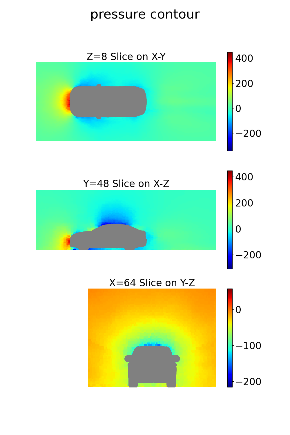
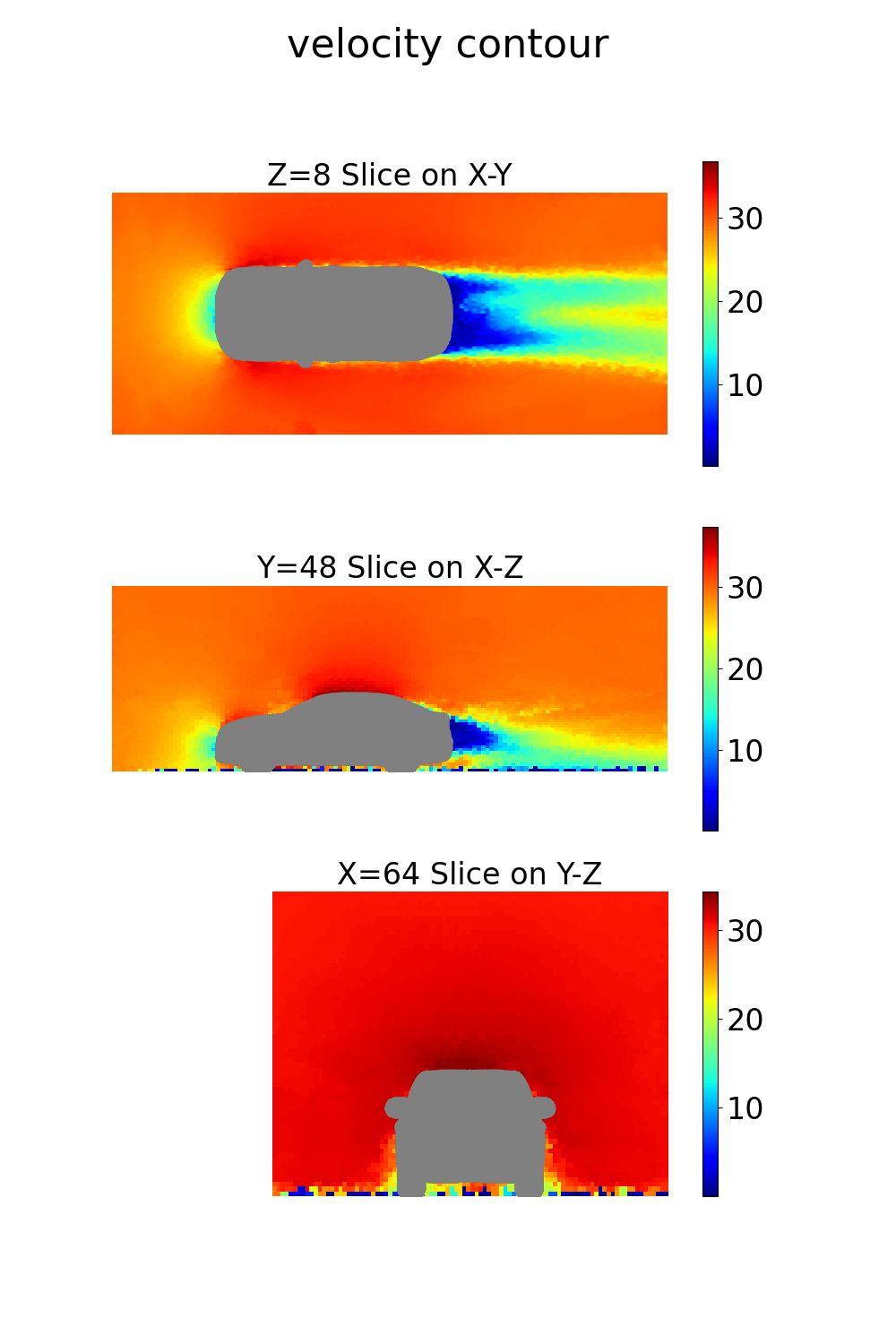
coordinates: 3D coordinates of points in the volume around the vehiclevelocity: Velocity vector (u, v, w components) at each point in the volumepressure: Pressure values at each point in the volumeturbulent_kinetic_energy: Turbulent kinetic energy at each volume pointturbulent_viscosity: Turbulent viscosity at each volume pointsdf: Signed distance field values at each point
Surface Field Predictions:
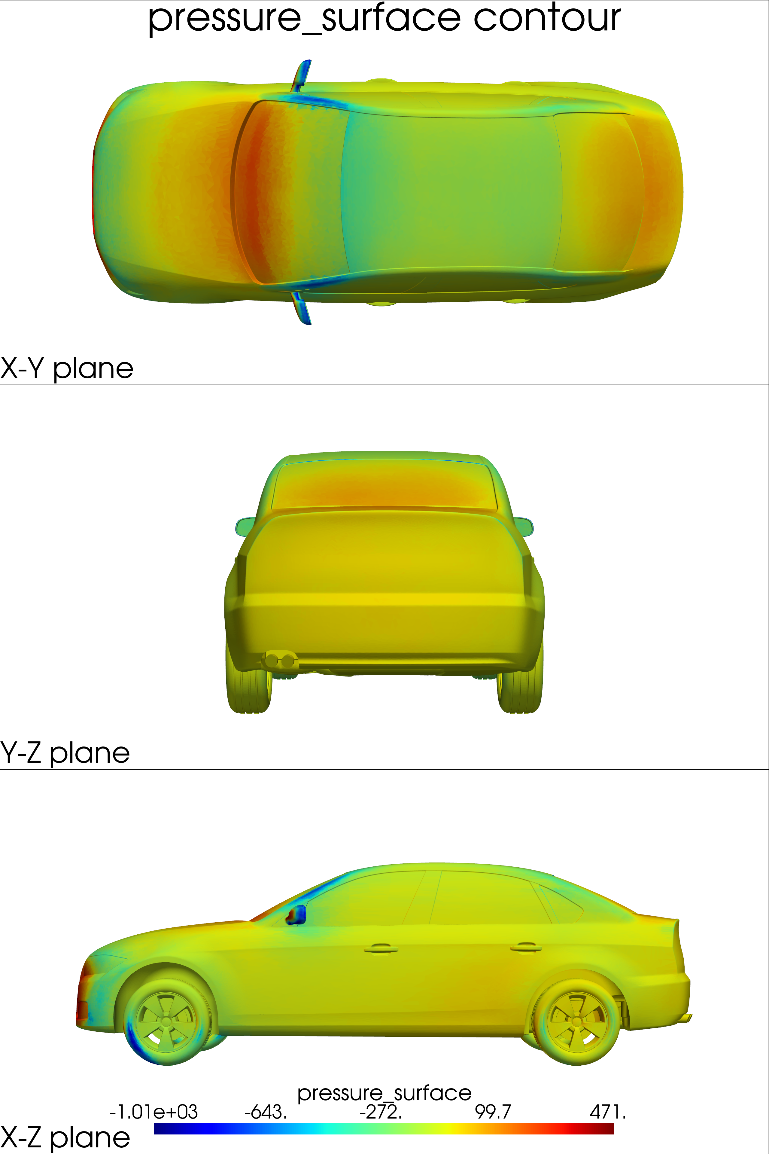
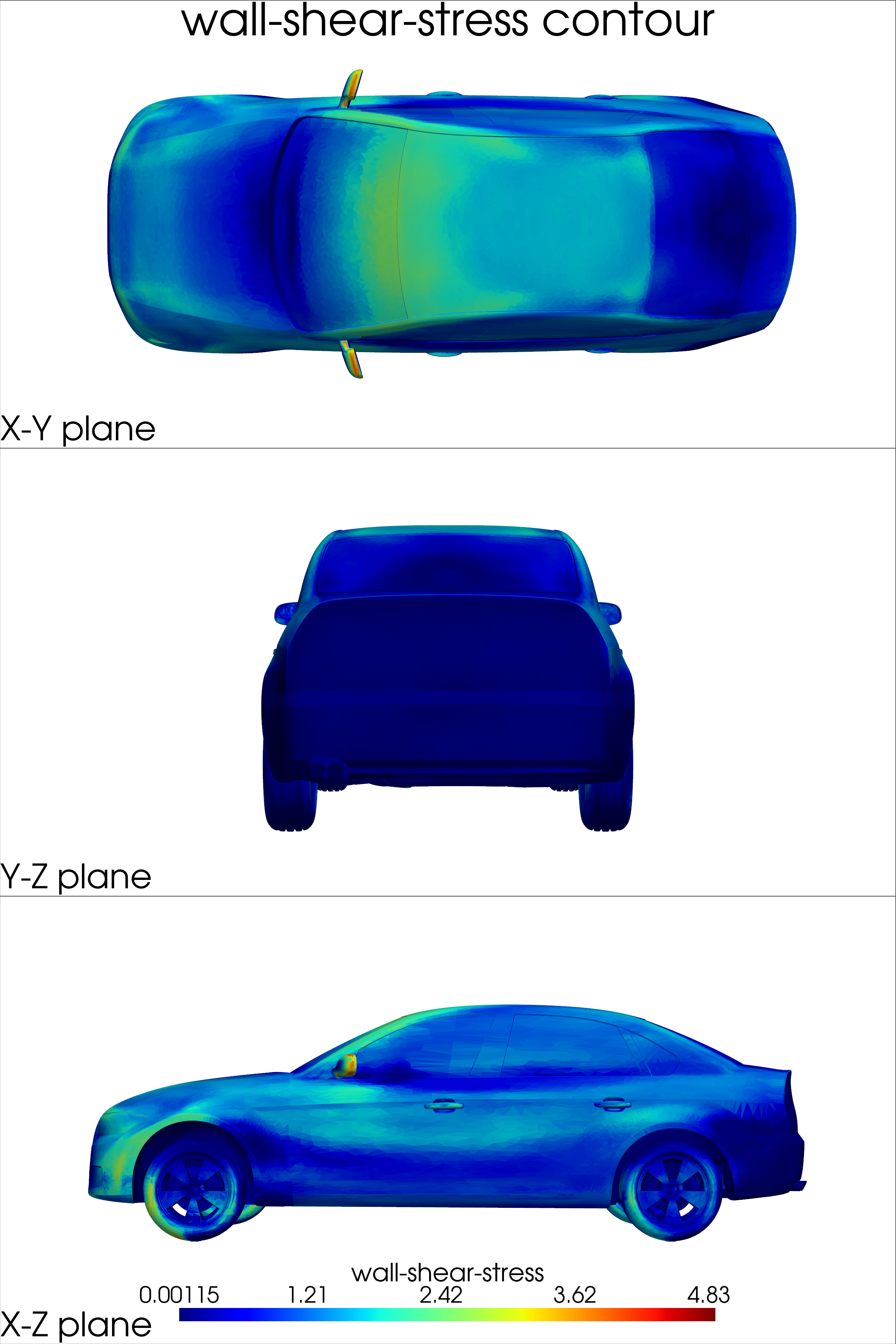
surface_coordinates: 3D coordinates of points on the vehicle surfacepressure_surface: Pressure values on the vehicle surfacewall_shear_stress: Wall shear stress values on the surface
Global Quantities:
drag_force: Total aerodynamic drag force on the vehiclelift_force: Total aerodynamic lift force on the vehiclebounding_box_dims: Dimensions of the computational domain
Surface predictions are computed at each cell of the input mesh and can be visualized directly on the vehicle surface. Volume predictions are computed on a point cloud around the vehicle and can be used to visualize flow features in the surrounding air volume. The exact number of prediction points for volume quantities is controlled by the point_cloud_size parameter.
Note
The /v1/infer endpoint computes both volume and surface predictions. Additionally, the /v1/infer/surface and /v1/infer/volume endpoints are available for computing surface and volume solutions separately.
Note
Use the /v1/model/config endpoint to retrieve the configuration settings used for model training and inference.
Note
For a list of available endpoints, see the API Reference.
Important
Refer to the performance data for estimated inference speeds on different GPU models.
Post Processing#
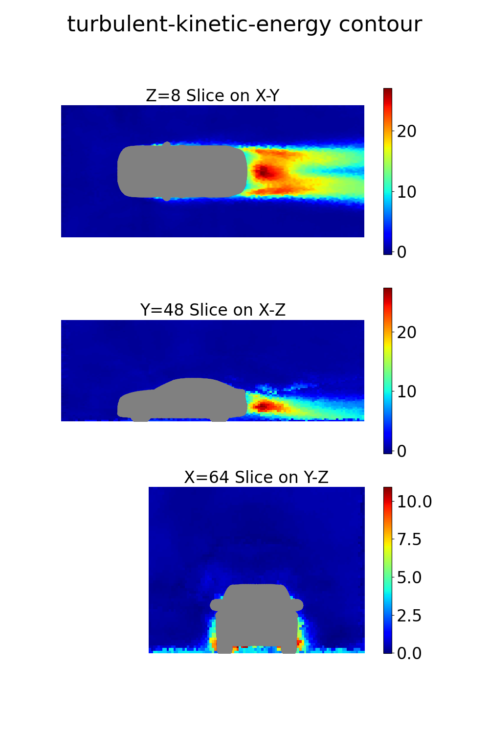
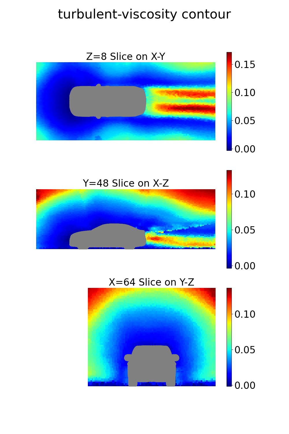
The final step is to perform some basic visualization of the results. The NIM provides both surface and volume field predictions that can be visualized using Python libraries like PyVista. Here’s an example script to visualize the volume and surface quantities:
import numpy as np
import pyvista as pv
import matplotlib.pyplot as plt
from scipy.interpolate import griddata
import copy
import os
import vtk

vtk.vtkObject.GlobalWarningDisplayOff()
os.environ["NO_AT_BRIDGE"] = "1"

pv.start_xvfb()

# Define the volume plotting function
def volume_plot(mesh, out_dict, coordinates, bounding_box_dims, grid_resolution):

    # Iterate over the keys of the output dictionary
    for j in out_dict.keys():
        field_name = j
        field_data = out_dict[j]

        if field_data.shape[1] == 1:
            field_data_cells = field_data
        else:
            field_data_cells = np.expand_dims(
                np.sqrt(np.sum(np.square(field_data), 1)), -1
            )

        x = coordinates[:, 0]
        y = coordinates[:, 1]
        z = coordinates[:, 2]

        grid_x, grid_y, grid_z = np.meshgrid(
            np.linspace(
                bounding_box_dims[0][0], bounding_box_dims[1][0], grid_resolution[0]
            ),
            np.linspace(
                bounding_box_dims[0][1], bounding_box_dims[1][1], grid_resolution[1]
            ),
            np.linspace(
                bounding_box_dims[0][2], bounding_box_dims[1][2], grid_resolution[2]
            ),
        )

        # Interpolate the field onto the grid
        field_interp = griddata(
            (x, y, z), field_data_cells, (grid_x, grid_y, grid_z), method="nearest"
        )
        field_interp = np.transpose(field_interp, (1, 0, 2, 3))

        fig, axes = plt.subplots(3, 1, figsize=(10, 15))
        fig.suptitle(f"{field_name} contour", fontsize=32)
        # XY
        idx = int(grid_resolution[2] / 8)
        field_plot = copy.deepcopy(field_interp[:, :, idx])
        field_plot = field_plot.T
        field_plot = field_plot[0]
        im = axes[0].imshow(
            field_plot,
            extent=(
                bounding_box_dims[0][0],
                bounding_box_dims[1][0],
                bounding_box_dims[0][1],
                bounding_box_dims[1][1],
            ),
            origin="lower",
            cmap="jet",
            aspect="equal",
            vmax=np.ma.masked_invalid(field_plot).max(),
            vmin=np.ma.masked_invalid(field_plot).min(),
        )
        axes[0].axis("off")

        # Add a horizontal colorbar
        cbar = fig.colorbar(im, ax=axes[0], orientation="vertical")
        cbar.ax.tick_params(labelsize=24)
        axes[0].set_xlabel("X (m)")
        axes[0].set_ylabel("Y (m)")
        axes[0].set_title(f"Z={idx} Slice on X-Y", fontsize=24)

        # Overlay the STL vertices
        stl_vertices = np.array(mesh.points)
        axes[0].scatter(
            stl_vertices[:, 0], stl_vertices[:, 1], c="grey", s=50, label="STL Geometry"
        )

        # XZ
        idx = int(grid_resolution[1] / 2)
        field_plot = copy.deepcopy(field_interp[:, idx, :])
        field_plot = field_plot.T
        field_plot = field_plot[0]
        im = axes[1].imshow(
            field_plot,
            extent=(
                bounding_box_dims[0][0],
                bounding_box_dims[1][0],
                bounding_box_dims[0][2],
                bounding_box_dims[1][2],
            ),
            origin="lower",
            cmap="jet",
            aspect="equal",
            vmax=np.ma.masked_invalid(field_plot).max(),
            vmin=np.ma.masked_invalid(field_plot).min(),
        )
        axes[1].axis("off")

        # Add a horizontal colorbar
        cbar = fig.colorbar(im, ax=axes[1], orientation="vertical")
        cbar.ax.tick_params(labelsize=24)
        axes[1].set_xlabel("X (m)")
        axes[1].set_ylabel("Z (m)")
        axes[1].set_title(f"Y={idx} Slice on X-Z", fontsize=24)

        # Overlay the STL vertices
        stl_vertices = np.array(mesh.points)
        axes[1].scatter(
            stl_vertices[:, 0], stl_vertices[:, 2], c="grey", s=50, label="STL Geometry"
        )

        # YZ
        idx = int(grid_resolution[0] / 2)
        field_plot = copy.deepcopy(field_interp[idx, :, :])
        field_plot = field_plot.T
        field_plot = field_plot[0]
        im = axes[2].imshow(
            field_plot,
            extent=(
                bounding_box_dims[0][1],
                bounding_box_dims[1][1],
                bounding_box_dims[0][2],
                bounding_box_dims[1][2],
            ),
            origin="lower",
            cmap="jet",
            aspect="equal",
            vmax=np.ma.masked_invalid(field_plot).max(),
            vmin=np.ma.masked_invalid(field_plot).min(),
        )
        axes[2].axis("off")

        # Add a horizontal colorbar
        cbar = fig.colorbar(im, ax=axes[2], orientation="vertical")
        cbar.ax.tick_params(labelsize=24)
        axes[2].set_xlabel("Y (m)")
        axes[2].set_ylabel("Z (m)")
        axes[2].set_title(f"X={idx} Slice on Y-Z", fontsize=24)

        # Overlay the STL vertices
        stl_vertices = np.array(mesh.points)
        axes[2].scatter(
            stl_vertices[:, 1], stl_vertices[:, 2], c="grey", s=50, label="STL Geometry"
        )

        # Save the figure to a PNG file
        os.makedirs("output", exist_ok=True)
        plt.savefig(f"output/{field_name}_slices.png")


# Define the surface plotting function
def surface_plot(mesh, out_dict):
    num_cells = mesh.n_cells
    for j in out_dict.keys():
        field_name = j
        field_data = out_dict[j]
        assert field_data.shape[0] == num_cells
        if field_data.shape[1] == 1:
            field_data_cells = field_data
        else:
            field_data_cells = np.expand_dims(
                np.sqrt(np.sum(np.square(field_data), 1)), -1
            )

        mesh.cell_data[field_name] = field_data_cells

        plotter = pv.Plotter(off_screen=True, window_size=[2560, 3840], shape=(3, 1))

        # Add title to the plot
        plotter.add_text(f"{field_name} contour", position="upper_edge", font_size=52)

        sargs = dict(position_x=0.2, title_font_size=72, label_font_size=64)

        plotter.subplot(0, 0)
        plotter.add_mesh(
            mesh,
            scalars=field_name,
            cmap="jet",
            preference="cell",
            show_scalar_bar=False,
        )  # preference set to cell
        plotter.camera_position = "xy"
        plotter.camera.zoom(1.8)
        plotter.add_text("X-Y plane", position=(0.5, 0.9), font_size=48)

        plotter.subplot(1, 0)
        plotter.add_mesh(
            mesh,
            scalars=field_name,
            cmap="jet",
            preference="cell",
            show_scalar_bar=False,
        )  # preference set to cell
        plotter.camera_position = "yz"
        plotter.camera.zoom(2.2)
        plotter.add_text("Y-Z plane", position=(0.5, 0.9), font_size=48)

        plotter.subplot(2, 0)
        plotter.add_mesh(
            mesh,
            scalars=field_name,
            cmap="jet",
            preference="cell",
            show_scalar_bar=True,
            scalar_bar_args=sargs,
        )  # preference set to cell
        plotter.camera_position = "xz"
        plotter.camera.zoom(1.8)
        plotter.add_text("X-Z plane", position=(0.5, 0.9), font_size=48)

        plotter.screenshot(f"{field_name}_contours.png")


# Define the plotting function
def plot_contours(mesh, out_dict, grid_resolution):

    if "pressure_surface" in out_dict.keys():
        surf_dict = {}
        surf_dict["pressure_surface"] = out_dict["pressure_surface"][0]
        surf_dict["wall-shear-stress"] = out_dict["wall_shear_stress"][0]
        surface_plot(mesh, surf_dict)

    if "pressure" in out_dict.keys():
        vel_dict = {}
        vel_dict["pressure"] = out_dict["pressure"][0]
        vel_dict["velocity"] = out_dict["velocity"][0]
        vel_dict["turbulent-kinetic-energy"] = out_dict["turbulent_kinetic_energy"][0]
        vel_dict["turbulent-viscosity"] = out_dict["turbulent_viscosity"][0]
        bounding_box_dims = out_dict["bounding_box_dims"]
        coordinates = out_dict["coordinates"][0]
        volume_plot(mesh, vel_dict, coordinates, bounding_box_dims, grid_resolution)
Save this code in a plot.py file, and use it in your request script:
import io, httpx, numpy
import pyvista as pv
from plot import plot_contours

url = "http://localhost:8000/v1/infer"
stl_file_path = 'drivaerml_single_solid_stls/drivaer_1_single_solid.stl'
data = {
    "stream_velocity": "30.0",
    "stencil_size": "1",
    "point_cloud_size": "500000",
}
with open(stl_file_path, "rb") as stl_file:
    files = {"design_stl": (stl_file_path, stl_file)}
    r = httpx.post(url, files=files, data=data, timeout=120.0)
if r.status_code != 200:
    raise Exception(r.content)
with numpy.load(io.BytesIO(r.content)) as output_data:
    output_dict = {key: output_data[key] for key in output_data.keys()}
print(output_dict.keys())

# Read the mesh file
mesh = pv.read(stl_file_path)

# Call the plotting function
plot_contours(
    mesh=mesh,
    out_dict=output_dict,
    grid_resolution=[128, 96, 64]
)
This will create .png files for surface and volume predictions.
Note
If the STL file contains a large number of cells, you might encounter warning messages regarding texture buffer size. These warnings are expected and do not impact the plotting process. To suppress them, add the following lines at the beginning of your plotting script:
import vtk
vtk.vtkObject.GlobalWarningDisplayOff()