FFT

Overview

FFT implements the Fourier Transform applied to 2D images, supporting real- and complex-valued inputs. It returns the image representation in the frequency domain. It is useful for content analysis based on signal frequencies, and enables image operations that are more efficiently performed on the frequency domain, among other uses.

Input in space domain	Magnitude spectrum

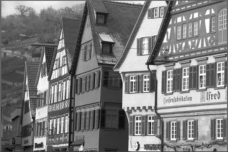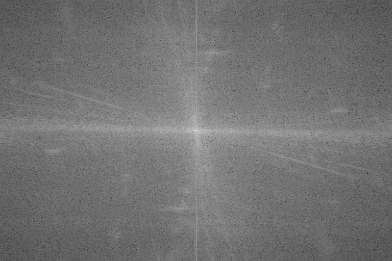Implementation

The FFT - Fast Fourier Transform is a divide-and-conquer algorithm for efficiently computing discrete Fourier transforms of complex or real-valued data sets in \(O(n \log n)\). It is one of the most important and widely used numerical algorithms in computational physics and general signal processing.

The Discrete Fourier Transform (DFT) generally maps a complex-valued vector \(x_k\) on the space domain into its frequency domain representation given by:

\[ I'[u,v] = \sum^{M-1}_{m=0} \sum^{N-1}_{n=0} I[m,n] e^{-2\pi i (\frac{um}{M}+\frac{vn}{N})} \]

Where:

• \(I\) is the input image in spatial domain
• \(I'\) is its frequency domain representation
• \(M\times N\) is input's dimensions

Note that the \(I'\) is left denormalized as the spectrum is eventually normalized in subsequent stages of the pipeline (if at all).

Depending on image dimension, different techniques are employed for best performance:

• CPU backend
  • Fast paths when \(M\) or \(N\) can be factored into \(2^a \times 3^b \times 5^c\)
• CUDA backend
  • Fast paths when \(M\) or \(N\) can be factored into \(2^a \times 3^b \times 5^c \times 7^d\)

In general the smaller the prime factor is, the better the performance, i.e., powers of two are fastest.

FFT supports the following transform types:

• complex-to-complex, C2C
• real-to-complex, R2C.

Data Layout

Data layout depends strictly on the transform type. In case of general C2C transform, both input and output data shall be of type VPI_IMAGE_FORMAT_2F32 and have the same size. In R2C mode, each input image row \((x_1,x_2,\dots,x_N)\) with type VPI_IMAGE_FORMAT_F32 results in an output row \((X_1,X_2,\dots,X_{\lfloor\frac{N}{2}\rfloor+1})\) of non-redundant complex elements with type VPI_IMAGE_FORMAT_2F32. In both cases, input and output image heights are the same.

FFT type	input		output
	type	size	type	size
C2C	VPI_IMAGE_FORMAT_2F32	\(W \times H\)	VPI_IMAGE_FORMAT_2F32	\(W \times H\)
R2C	VPI_IMAGE_FORMAT_F32	\(W \times H\)	VPI_IMAGE_FORMAT_2F32	\(\big( \lfloor\frac{W}{2}\rfloor+1 \big) \times H\)

For real inputs, the output contains only the non-redundant elements, thus only the left half of spectrum returned. In order to retrieve the whole Hermitian (symmetric-conjugate) output, the right half must be completed so that the following conditions are met:

\begin{align*} F_{\textbf{re}}(u,v) &= F_{\textbf{re}}(-u,-v) \\ F_{\textbf{re}}(-u,v) &= F_{\textbf{re}}(u,-v) \\ F_{\textbf{im}}(u,v) &= -F_{\textbf{im}}(-u,-v) \\ F_{\textbf{im}}(-u,v) &= -F_{\textbf{im}}(u,-v) \end{align*}

The following diagram shows how this is accomplished:

Completing the output spectrum

The zero-th element in spectrum output represents the DC (0 Hz) component. Usually for visualization it's preferred that DC is at the center. One way to accomplish this is to shift the 4 quadrants around as shown in the diagram below:

\(Q_0\) \(Q_1\) \(Q_2\) \(Q_3\)

\(\rightarrow\)

\(Q_3\) \(Q_2\) \(Q_1\) \(Q_0\)

Usage

1. Initialization phase
   1. Include the header that defines the image FFT function and the needed image format conversion functionality.

      #include <vpi/algo/ConvertImageFormat.h>
      #include <vpi/algo/FFT.h>

   2. Define the input image object.

          VPIImage input = /*...*/;

   3. Create the output image that will hold the spectrum. Since input is real, only non-redundant values will be calculated and output width is \(\lfloor \frac{w}{2} \rfloor+1\).

          uint32_t w, h;
          vpiImageGetSize(input, &w, &h);
       
          VPIImage spectrum;
          vpiImageCreate(w / 2 + 1, h, VPI_IMAGE_FORMAT_2F32, 0, &spectrum);

   4. Create the temporary image that stores the floating-point representation of the input image. Also allocates host memory to hold the full Hermitian representation, calculated from VPI's output.

          VPIImage inputF32;
          vpiImageCreate(w, h, VPI_IMAGE_FORMAT_F32, 0, &inputF32);
       
          float *tmpBuffer = (float *)malloc(w * 2 * h * sizeof(float));

   5. Create the FFT payload on the CUDA backend. Input is real and output is complex. Problem size refers to input size.

          VPIPayload fft;
          vpiCreateFFT(VPI_BACKEND_CUDA, w, h, VPI_IMAGE_FORMAT_F32, VPI_IMAGE_FORMAT_2F32, &fft);

   6. Create the stream where the algorithm will be submitted for execution.

          VPIStream stream;
          vpiStreamCreate(0, &stream);

2. Processing phase
   1. Convert the input to floating-point using CUDA, keeping the input range the same.

          vpiSubmitConvertImageFormat(stream, VPI_BACKEND_CUDA, input, inputF32, VPI_CONVERSION_CAST, 1, 0);

   2. Submit the FFT algorithm to the stream, passing the floating-point input and the output buffer. Since the payload was created on the CUDA backend, it'll use CUDA for processing.

          vpiSubmitFFT(stream, fft, inputF32, spectrum, 0);

   3. Wait until the processing is done.

          vpiStreamSync(stream);

   4. Now on to the result. First lock the spectrum data.

          VPIImageData data;
          vpiImageLock(spectrum, VPI_LOCK_READ, &data);

   5. Convert the complex frequency data into magnitude ready to get displayed.
      1. Fills the right half of the complex data with the missing values. The left half is copied directly from VPI's output.

             // make width/height even
             w = w & -2;
             h = h & -2;
          
             // center pixel coordinate
             int cx = w / 2;
             int cy = h / 2;
          
             for (int i = 0; i < (int)h; ++i)
             {
                 for (int j = 0; j < (int)w; ++j)
                 {
                     float re, im;
                     if (j < cx)
                     {
                         const float *pix =
                             (const float *)((const char *)data.planes[0].data + i * data.planes[0].pitchBytes) + j * 2;
                         re = pix[0];
                         im = pix[1];
                     }
                     else
                     {
                         const float *pix =
                             (const float *)((const char *)data.planes[0].data + ((h - i) % h) * data.planes[0].pitchBytes) +
                             ((w - j) % w) * 2;
                         // complex conjugate
                         re = pix[0];
                         im = -pix[1];
                     }
          
                     tmpBuffer[i * (w * 2) + j * 2]     = re;
                     tmpBuffer[i * (w * 2) + j * 2 + 1] = im;
                 }
             }

      2. Convert the complex frequencies into normalized log-magnitude

             float min = FLT_MAX, max = -FLT_MAX;
          
             for (int i = 0; i < (int)h; ++i)
             {
                 for (int j = 0; j < (int)w; ++j)
                 {
                     float re, im;
                     re = tmpBuffer[i * (w * 2) + j * 2];
                     im = tmpBuffer[i * (w * 2) + j * 2 + 1];
          
                     float mag            = logf(sqrtf(re * re + im * im) + 1);
                     tmpBuffer[i * w + j] = mag;
          
                     min = mag < min ? mag : min;
                     max = mag > max ? mag : max;
                 }
             }
          
             for (int i = 0; i < (int)h; ++i)
             {
                 for (int j = 0; j < (int)w; ++j)
                 {
                     tmpBuffer[i * w + j] = (tmpBuffer[i * w + j] - min) / (max - min);
                 }
             }

      3. Shift the spectrum so that DC is at center

             for (int i = 0; i < (int)h; ++i)
             {
                 for (int j = 0; j < (int)cx; ++j)
                 {
                     float a = tmpBuffer[i * w + j];
          
                     // quadrant 0?
                     if (i < cy)
                     {
                         // swap it with quadrant 3
                         tmpBuffer[i * w + j]               = tmpBuffer[(i + cy) * w + (j + cx)];
                         tmpBuffer[(i + cy) * w + (j + cx)] = a;
                     }
                     // quadrant 2?
                     else
                     {
                         // swap it with quadrant 1
                         tmpBuffer[i * w + j]               = tmpBuffer[(i - cy) * w + (j + cx)];
                         tmpBuffer[(i - cy) * w + (j + cx)] = a;
                     }
                 }
             }

   6. As VPI output image isn't needed anymore, just unlock it

          vpiImageUnlock(spectrum);

   7. Now display tmpBuffer using your preferred method.
3. Cleanup phase
   1. Free resources held by the stream, the payload, the input and output images and the temporary host buffer.

          vpiStreamDestroy(stream);
          vpiPayloadDestroy(fft);
          vpiImageDestroy(input);
          vpiImageDestroy(inputF32);
          vpiImageDestroy(spectrum);
          free(tmpBuffer);

For more details, consult the FFT API reference.

Limitations and Constraints

Constraints for specific backends supersede the ones specified for all backends.

All Backends

• The following input image formats are accepted:
  • VPI_IMAGE_FORMAT_F32 - real input.
  • VPI_IMAGE_FORMAT_2F32 - complex input.
• The following output image formats are accepted:
  • VPI_IMAGE_FORMAT_2F32 - complex output.

CPU

• If input has format VPI_IMAGE_FORMAT_F32, its width must be even.
• Input and output rows must be aligned to 4 bytes.

CUDA

• There can be memory allocation in first call to vpiSubmitFFT and every time the input or output row stride changes with respect to previous call.

PVA and VIC

• Not implemented.

Performance

For information on how to use the performance table below, see Algorithm Performance Tables.
Before comparing measurements, consult Comparing Algorithm Elapsed Times.
For further information on how performance was benchmarked, see Performance Measurement.

clear filters Device: Jetson AGX Xavier Jetson TX2 Jetson Nano  -  Streams: 1 4 8