Technical Brief#
Overview#
One of the biggest challenges in the commercial fleet industry is routing optimization. This is prevalent in many industries, where determining the most cost-effective route can contribute significant cost savings for meal delivery where a single restaurant franchise can deliver millions of meals a day, or a telecommunications company that dispatches millions of jobs per year. In these types of large scale scenarios, inefficient routes can cost billions of dollars in operational costs as well as reduce our environmental carbon footprint. A computational solver can minimize these inefficiencies by finding the most optimal routes across a list of locations. Computational CPU based solvers are available today but using the massive throughput of GPU acceleration, more ambitious algorithms will help fuel our future.
Route optimization problems such as those described above are commonly known as the Traveling Salesperson (TSP) problem. To reduce the time to develop a GPU accelerated TSP solution, NVIDIA has developed the route optimization AI workflow to streamline development of Vehicle Routing Problem (VRP) solutions.
This NVIDIA AI workflow contains details on how to deploy a sample opinionated AI solution for route optimization; the following items are included:
Origin-destination cost-matrix creation
Data preprocessing
NVIDIA cuOpt™ GPU accelerated solver pipeline
Driving directions
Map visualization
Components for authentication, logging and monitoring the workflow
Cloud Native deployable bundle packaged as a helm chart
Note
The components and instructions used in the workflow are intended to be used as examples for integration, and may not be sufficiently production-ready on their own as stated. The workflow should be customized and integrated into one’s own infrastructure, using the workflow as reference.
This AI workflow covers three different TSP use cases:
- Last Mile Delivery (LMD)
Fleet of trucks are dispatched from distribution centers to deliver orders to stores.
- Pickup and Delivery (PDP)
Fleet of trucks are dispatched but then fulfills orders by picking them up and dropping them off to a different location. For example, a DoorDash driver picks up a food order from a restaurant and delivers it to the customer’s home address.
- Dispatch Optimization
Service provider is dispatched to fulfill a list of different service requests. These are allocated a certain amount of time per service request and the time can vary according to request. For example, a telecommunications technician is assigned to a customer’s home to install a router and then to a different home to install a data cable.
Using the above assets, this NVIDIA AI workflow provides a reference for you to get started and build your own AI solution with minimal preparation and includes enterprise-ready implementation best practices which range from authentication, monitoring, reporting, and load balancing, helping you achieve the desired AI outcome more quickly while still allowing a path for you to deviate.
NVIDIA AI workflows are designed as microservices, which means they can be deployed on Kubernetes alone or with other microservices to create a production-ready application for seamless scaling in your Enterprise environment.
The workflow components are packaged together into a deployable solution described in the diagram below
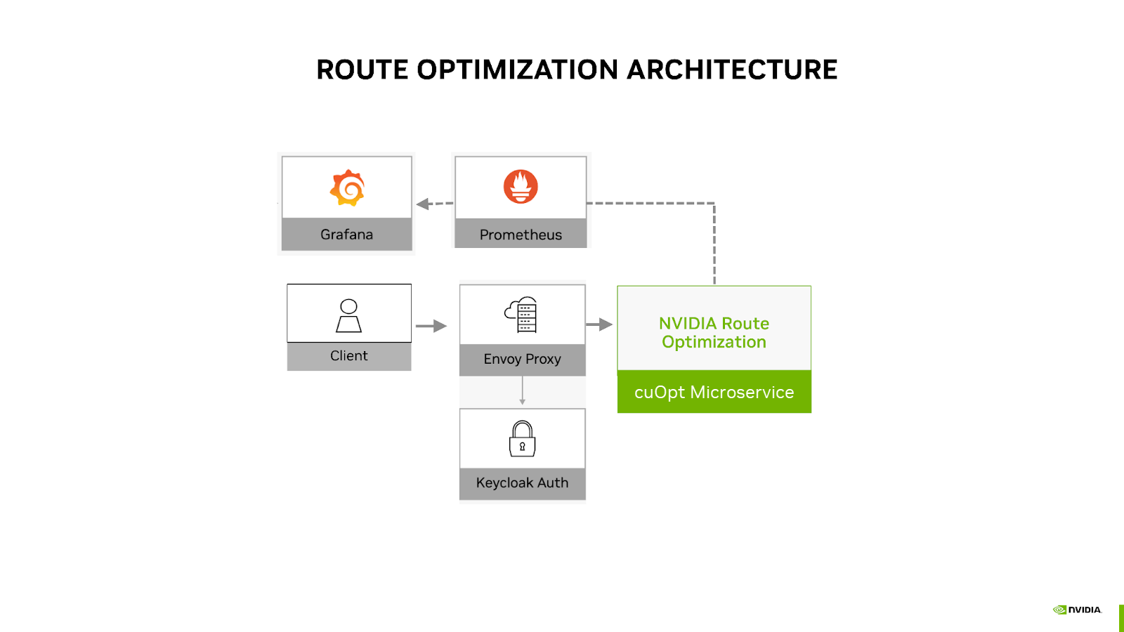
These components are used to build and deploy route optimization cuOpt microservice, integrated together with the additional components as indicated in the diagram below:
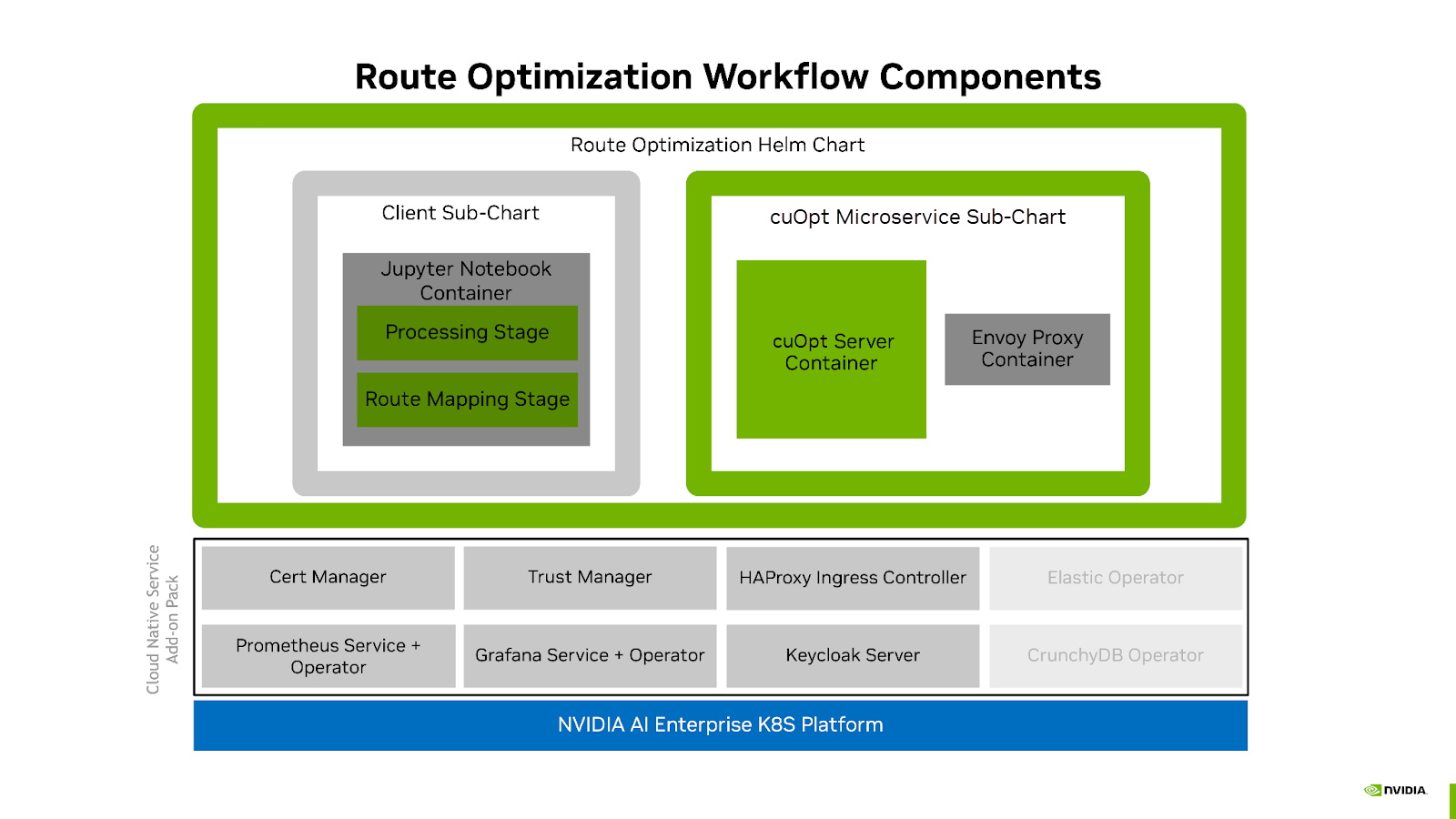
More information about the components used can be found in the route optimization and the NVIDIA Cloud Native Service Add-on Pack Deployment Guide.
Furthermore, the route optimization AI workflow describes how to integrate the cuOpt Server API with third party APIs for route mapping and map visualization.
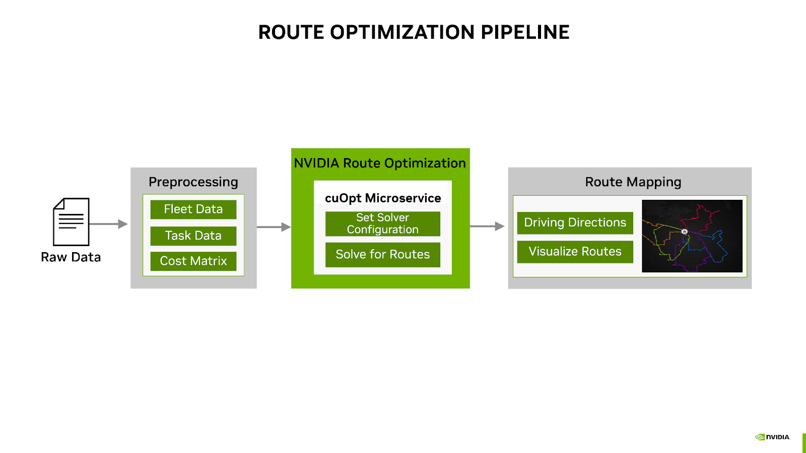
NVIDIA AI Workflow Components#
The NVIDIA route optimization AI workflow uses the NVIDIA cuOpt server via a representational state transfer (REST) microservice API to generate routes. To do this, a series of sample synthetic datasets are included within the workflow to assign a set of orders to a fleet of delivery drivers. Three csv files are used by workflow to assign the drivers to their appropriate orders; Orders, Depot and Route.
cuOpt Managed Service#
While previously available as an SDK, cuOpt is now available as a cloud service. Instead of installing the Python SDK or deploying the microservice themselves, (either locally or in the cloud), customers can more quickly adopt cuOpt GPU accelerated route solvers within their Route Optimization applications. Since the cuOpt Managed Service has built-in authentication, scaling, and other mechanisms, customers can use cuOpt without setting it up themselves. Now, customers can access the client by getting credentials and an API endpoint. Users can go through data preprocessing themselves, save all the data to one JSON file, and send this JSON file in one command to the cuOpt solver. The cuOpt solver will return the results which can either be printed or saved to a new JSON file to be processed later. After getting the initial results, customers can update the JSON file with new data (for example, new orders that have been placed or an updated cost matrix) and send the new JSON file to cuOpt to get the reoptimized routes.
Sample Datasets#
A series of sample synthetic datasets are included within the workflow to assign orders to a fleet of delivery drivers. Three CSV files are used in each use case to assign the drivers to their appropriate orders; Orders, Depot and Routes. The following paragraphs describe each of these synthetic datasets further and on how they are used for each of the specific use cases.
- Order
An Order can be a delivery to a customer, a pickup from a customer, or some other type of work. Examples include a furniture delivery, a grease pickup from a restaurant, or an inspection visit. In this workflow, we look at deliveries from a distribution center to stores. The Order dataset includes the stores’ data. This includes store name, location, start and end time (store hours), demand (order weight in pounds), and service time (how long it will take to unload the package).
- Depot
A Depot is a location that a vehicle departs from at the beginning of its workday and returns to at the end of the workday. Depots are locations where the vehicles are loaded (for deliveries) or unloaded (for pickups). In some cases, a depot can also act as a renewal location whereby the vehicle can unload or reload and continue performing deliveries and pickups. A Depot has open and close times, as specified by a hard time window. Vehicles can’t arrive at a Depot outside this time window. In this Route Optimization workflow, vehicles depart the depot in the morning and return at the end of day. The depots’ information includes name, location, and start and end time (operation hours).
- Route
Route information specifies the vehicle and driver characteristics, such as the vehicle capacity, work shift hours, and driving range, and it represents the traversal between depots and orders. The features needed here are vehicle name/ID number, start and end depot name, start and end time (vehicle/driver shift hours), and carrying capacity.
The sample AI workflow uses a combination of these three CSVs to find the best cost-effective route using your data for your specific use case. For example, within the Order CSV file, the package weight is indicated, and the Route CSV contains the route of the delivery truck with the maximum order weight. The Route is assigned to a Depot.
Note
You might have additional features depending on the problem, such as order priorities or vehicle break time windows. Other features would be preprocessed similarly to the features shown in the workflow.
Solver Configuration
The last piece of data that needs to be sent to the cuOpt solver is the configuration settings. The two main settings are time limit and number of climbers.
The time limit is the maximum time allotted to find a solution. This depends on the user, who has the flexibility of setting a higher time limit for better results. The number of climbers is the number of parallel agents examining the solution search space.
If the user wants the first solution, then around 2-3 seconds for 2000-4000 climbers is enough.
By default, the number of climbers is chosen by considering the occupancy of a small GPU and experimented runtime vs the number of climbers trade-off (that is, the best result in the shortest time). Normally 1024 or multiple is a good start.
In some cases, like package delivery services, there are thousands of locations. In such cases, routes are generated overnight so cost matrices can be generated in time and the solver has a sufficient amount of time to get the optimized routes. However, orders can change during the day; new orders can be added, and existing orders can be delayed or lost. With such a large problem space, locations can be submitted to cuOpt in batches. When there’s a queue, we can give cuOpt solver a short time limit to reoptimize the initial routes and thus complete more jobs promptly such that drivers can obtain these new routes in real-time.
Jupyter Notebook Client#
As a part of the workflow, we provide a Jupyter Notebook to perform the data preprocessing and route mapping steps.
Data Preprocessing
The cuOpt server has a set of data requirements which are handled in the pre-processing stage that includes modeling the data as arrays of integers and creating a cost matrix. In this route optimization AI workflow, a cost matrix has already been built for you and is provided as a csv file. The cost matrix represents the travel time from one depot or order to another. Once the preprocessing stage is complete, the data from the three datasets mentioned above as well as the cost matrix are sent over and imported to the cuOpt Server.
Note that when there is a mixed fleet of vehicles, where different transportation types may have different travel times, additional cost matrices may be required. For example, a single cost matrix can be used in the LMD use case for both trucks and EV vans since these two vehicle types have the same travel time. But in the PDP use cases where cars and bicycles are used for transporting deliveries, more than one cost matrix is required since the two vehicle types have different travel times.
The cost matrix example below has five total locations. The cost matrix will look like this in the form of a dataframe.
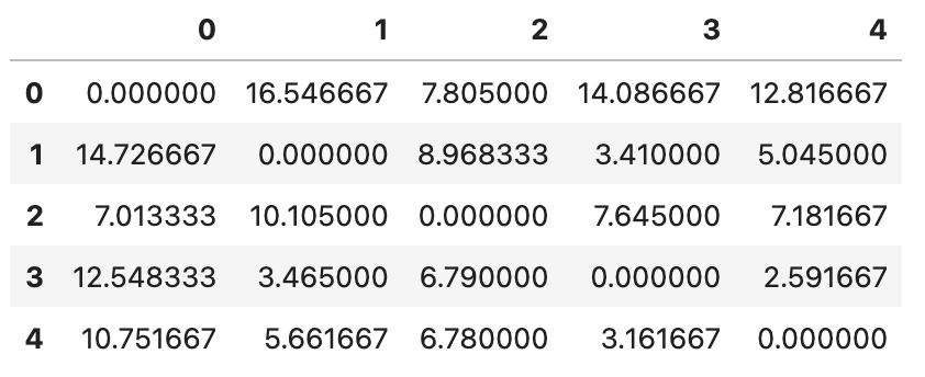
The above cost matrix represents the travel time in minutes. Similar to our AI Workflow, the travel time from location 0 to location 1 takes 16.546667 minutes.
Note
The cost of going from a location to itself is typically 0, and the cost of going from location A to location B is not necessarily equal to going from location B to location A.
Once the preprocessing stage is complete, the order, depot and route data as well as the cost matrix, are sent over and imported to the cuOpt Server via API calls. These calls are made using the Jupyter Notebook client.
Route Mapping
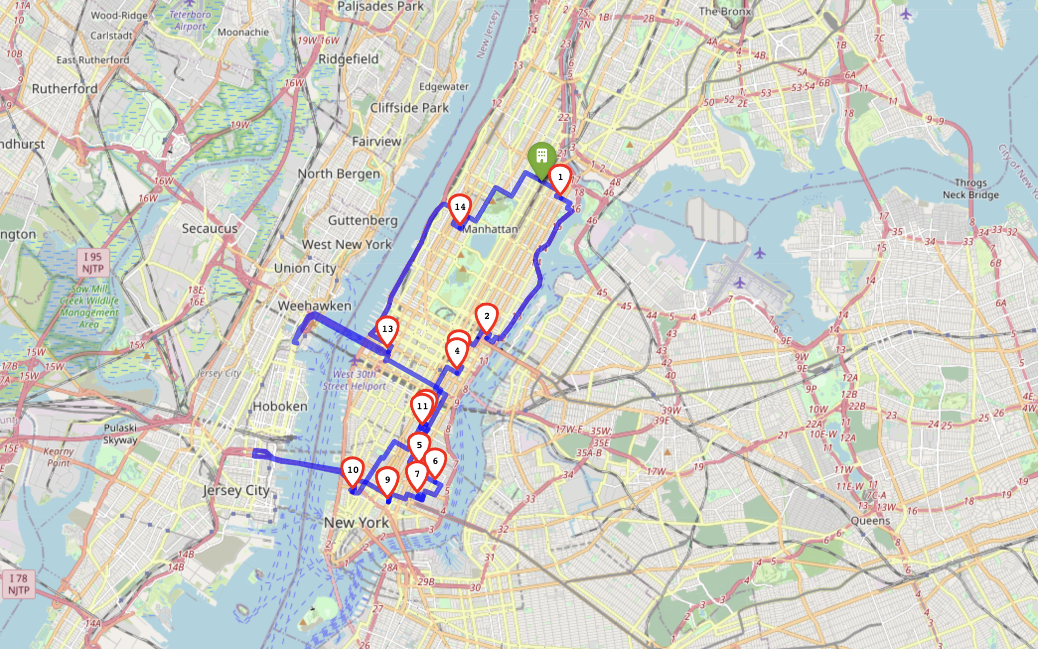
Once the cuOpt solver returns-optimized routes, the route optimization AI workflow uses the Open Source Routing Machine (OSRM) API as an open-source router which uses OpenStreetMap. OSRM parses the cuOpt solver response, converts locations to coordinate points and then maps the routes. These optimized routes inherently include driving directions for each order.
Additional Components#
Monitoring
Prometheus is an open-source monitoring and alerting solution. In this workflow, it stores pipeline performance metrics from Triton, which enables System Administrators to understand the health and throughput of the system.
While the metrics are available in plain text, Grafana is also used for visualization of the metrics via a dashboard. Some of the metrics available, for example, are shown below; depending on the usage metrics, the cuOpt pods can be scaled manually or automatically.