3. Compute Triage Guide

This guide provides a top-to-bottom triage workflow for CUDA kernel performance issues on NVIDIA GPUs using Nsight Compute.

3.1. Introduction

Use this guide when a CUDA kernel, graph or range are slower than expected and limit your overall application performance.

Some general guidelines for profiling CUDA:

• Keep capture settings stable while comparing runs.

• Start with the most minimal but representative workload.

• Ensure source correlation is available for source-page diagnosis. Compile with -lineinfo, run ncu --import-source on, and use --set full when source-level analysis is needed.

Apply this iterative optimization plan:

• Use Nsight Systems first if kernel priority is unclear, then use Nsight Compute.

• Focus on the single largest current limiter first.

• Do not optimize from a single metric in isolation.

• Apply one targeted refactor at a time.

• Re-profile immediately and keep or revert based on measured impact.

• Validate every change against absolute kernel duration. SOL percentages can drop while the kernel gets faster (e.g. when total work is reduced), so duration is the ground truth, not SOL %.

• Re-evaluate the dominant limiter on each new GPU generation: memory bandwidth tends to grow faster than SM count, so a kernel that saturated the bus on an older GPU may underperform on a newer one without modification.

• Stop when expected gains are small relative to complexity and risk.

For more detailed usage guidelines, see Usage Guidelines.

3.2. Triage Workflow

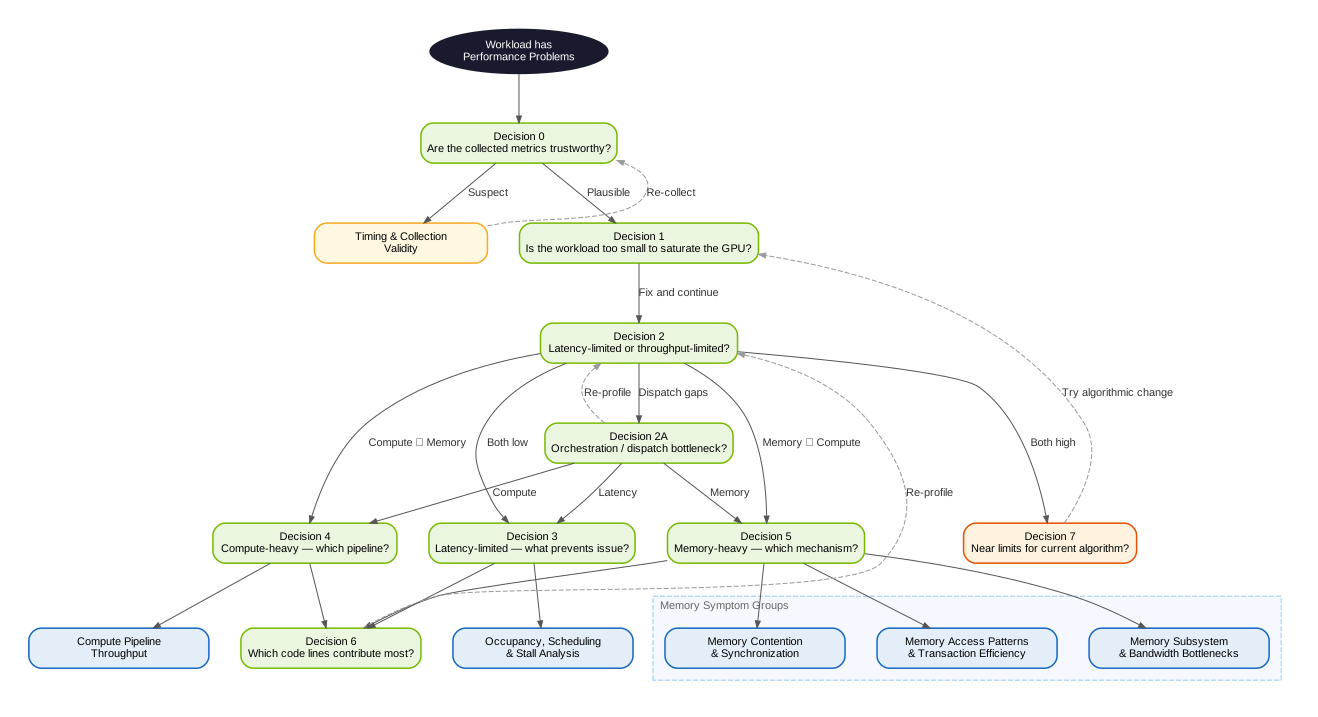
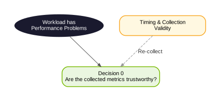
3.2.1. Decision 0: Are the collected metrics trustworthy?

Primary check	Look for
Kernel duration compares to Nsight Systems timing. Divergence beyond ~2× warrants investigation of clock/cache-control or replay-mode effects.	GPU Speed Of Light Throughput: Kernel duration (gpu__time_duration.sum) vs Nsight Systems wall-time.
All metric values are within logical range. Metrics don’t contradict each other (e.g. high throughput with zero issue activity).	Any pct_of_peak_sustained_* metric significantly above 100% [1] or negative.
Profiling configuration matches the analysis goal. Default kernel replay with clock locking is appropriate for isolated kernel analysis. Range or application replay with –clock-control none and –cache-control none is needed for system-representative behavior.	Session page Launch Settings
Profiled binary is release-optimized and was built with line-table info. Debug builds change code generation and timings; missing line tables prevent source-level attribution because metrics are collected at the SASS level.	Compile flags / build configuration: Verify -O2/release flags and nvcc -lineinfo (HPC compilers and Numba have equivalent options).

Next Actions:

• Metrics are suspect: Timing and Collection Validity (diagnose and fix collection issues, then re-collect and re-enter this decision).

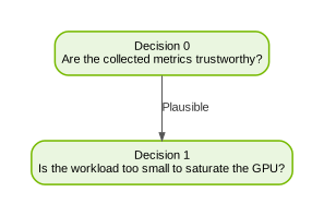
• Metrics look plausible: Decision 1: Is the workload too small to saturate the GPU?.

[1]

Small values slightly above 100% can be artifacts of multi-pass metric collection and do not constitute a blocking error. Only investigate when the overshoot is large or accompanied by other contradictory readings. See Metrics Overview.

3.2.2. Decision 1: Is the workload too small to saturate the GPU?

Primary checks	Look for
The grid does not fill all SMs at least once (less than one wave).	Launch Statistics: Waves per SM (launch__waves_per_multiprocessor < 1) Grid size (launch__grid_size) #SMs (launch__sm_count) [2]
Block size is not a multiple of 32 (warp size) Wastes threads in a partial warp.	Launch Statistics: Block size (launch__block_size)
Block size is very small Small block sizes can limit occupancy by exhausting the per-SM block slots, even when other resources like registers and shared memory are available. For common blocks/warps per SM limit configurations, fewer than 32 threads per block limits occupancy to 50%.	Launch Statistics: Block size (launch__block_size)
Achieved occupancy is below 60% unless the workload is dominated by Tensor Core usage, or compute or memory GPU SOL is already high. The grid does not expose enough parallelism to hide latency.	Occupancy: Achieved occupancy (sm__warps_active.avg.pct_of_peak_sustained_active)
The kernel runs in isolation, rather than concurrently with other kernels on the same GPU (multiple streams).	Timeline workload execution row

Next Actions:

• Workload too small:

  • Scale independent work across blocks first.

  • Typical refactor: parallelize independent outer-loop work across blocks instead of serializing it inside one block.

  • Re-profile before touching memory/pipeline micro-optimizations.

  • Confirm isolated workloads through range- or graph-level profiling in Nsight Compute, or with Nsight Systems.

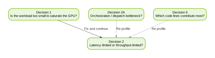
  • Then Decision 2: Is this latency-limited or throughput-limited?.

• Workload saturates the GPU: Decision 2: Is this latency-limited or throughput-limited?.

[2]

Note that launch__sm_count can be less than device__attribute_limits_num_sm when CUDA green contexts are used.

3.2.3. Decision 2: Is this latency-limited or throughput-limited?

Primary check	Look for	Next Actions
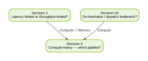
Compare SM Compute and Memory utilization.	GPU Speed Of Light Throughput: GPU Throughput Breakdown: sm__throughput​.avg.pct_of_peak_sustained_elapsed gpu__compute_memory_throughput​.avg.pct_of_peak_sustained_elapsed Below ~60%: low (latency-risk regime). Above ~80%: high (near-limit regime).	Both low: Decision 3: If latency-limited, what prevents instructions from issuing? Compute >> memory: Decision 4: If compute-heavy, which pipeline is the limiter? 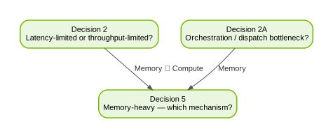Memory >> compute: Decision 5: If memory-heavy, which memory mechanism dominates? Both high: Decision 7: Are you close to hardware limits for this algorithm?
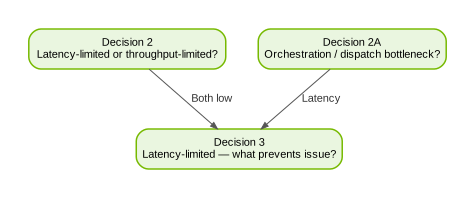
Issue activity indicates how often warps are issuing. Below ~20% indicates severe issue starvation.	Scheduler Statistics: smsp__issue_active.avg.pct_of_peak_sustained_active Compare with sm__throughput to separate issue-limited from pipe-limited cases.	Decision 3: If latency-limited, what prevents instructions from issuing?
Traffic may target system or peer memory instead of device DRAM.	Memory Workload Analysis/PM Sampling: Check when memory throughput is high but DRAM throughput is low — aperture traffic indicators and PCIe read/write bytes.	Symptom: Memory traffic is dominated by sysmem/peer apertures
Nsight Compute PM Sampling timeline shows dispatch/queue idle or sync gaps.	PM Sampling: Dispatch/Launch and SM Occupancy timeline rows; underfilled periods between dispatch start, block launch, and active compute.	Decision 2A: Is this an orchestration/dispatch bottleneck?

Note

If any utilization metric in this decision looks implausible (e.g. >100%, contradictory compute vs. memory readings), revisit Decision 0: Are the collected metrics trustworthy? and Timing and Collection Validity before routing further.

Occupancy-vs-Utilization:

Use this 2x2 framework to sharpen the branching decision when top-level throughputs are ambiguous:

• Low occupancy + low SM pipeline utilization

  Opportunity to launch more warps, overlap independent work, or increase arithmetic intensity per warp.

  Go to Decision 1: Is the workload too small to saturate the GPU? and Decision 3: If latency-limited, what prevents instructions from issuing?.
• Low occupancy + high SM pipeline utilization

  Launching extra warps is counter-productive because the busy pipe cannot absorb more work.

  Offload or reduce load on the dominant pipeline first.

  Go to Decision 4: If compute-heavy, which pipeline is the limiter?.
• High occupancy + low SM pipeline utilization

  Warps are present but not issuing — the workload is latency-bound.

  Go to Decision 3: If latency-limited, what prevents instructions from issuing? and check memory-latency indicators.
• High occupancy + high SM pipeline utilization

  SM is saturated. Reduce instruction count on the busiest pipeline, or restructure the algorithm.

  Go to Decision 4: If compute-heavy, which pipeline is the limiter? and Decision 7: Are you close to hardware limits for this algorithm?.

Practical thresholds:

• < 60% achieved occupancy is low

• >= 60% is high

• < 60% peak pipeline SOL is low

• >= 60% is high.

Note

Issue-slot utilization is the direct optimization target — not stall counts. A typical healthy kernel issues at ~0.5 instructions/cycle/scheduler. Stall reductions only translate to speedups when the kernel is actually latency-limited (see Decision 3: If latency-limited, what prevents instructions from issuing?).

Guardrail:

• For PM Sampling timeline views, treat top-level throughput rows as classifiers only; pick actions from constituent breakdown metrics and source-level contributors.

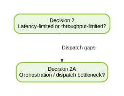
3.2.4. Decision 2A: Is this an orchestration/dispatch bottleneck?

Use this branch when Nsight Compute range PM Sampling rows indicate underfilled periods between dispatch start, block launch, and active compute, or when async queues spend visible time in wait/idle states.

Primary check	Look for
Dispatch-to-launch gap is a significant fraction of kernel active time.	PM Sampling: Launch and Dispatch timeline rows. Flag if Blocks Launched ramp-up is visibly slow relative to total kernel duration.
GPU idle or wait periods are excessive.	PM Sampling: SM Occupancy and Stalls timeline rows Flag if idle or wait periods occupy more than ~10% of the profiled range duration.
Compute and copy operations are fully serialized instead of overlapping.	PM Sampling: Launch and Dispatch timeline rows.

Next Actions:

• Orchestration/dispatch is the bottleneck (any check above is true):

  • Prioritize queue submission cadence, dependency ordering, and synchronization scope before kernel micro-optimization.

  • If host-side semaphore waits dominate idle time, investigate CPU-side submission latency and dependency scheduling to reduce GPU starvation.

  • Symptom: Nsight Compute PM Sampling shows dispatch/queue gaps for detailed timeline diagnosis.

  • Re-profile and return to Decision 2: Is this latency-limited or throughput-limited?.

• Orchestration looks healthy: continue with Decision 3: If latency-limited, what prevents instructions from issuing?, Decision 4: If compute-heavy, which pipeline is the limiter?, or Decision 5: If memory-heavy, which memory mechanism dominates? based on dominant limiter classification.

3.2.5. Decision 3: If latency-limited, what prevents instructions from issuing?

Primary check	Look for	Next Actions
Scheduler issue efficiency.	Scheduler Statistics: smsp__issue_active.avg.per_cycle_active < 0.5 is flagged as issue-starved. < 0.2 is severely starved.	Disambiguate memory-latency vs compute-dominated execution
Many warps are active but few are eligible to issue. Indicates dependency or synchronization stalls. Ratio below ~0.5 is a strong latency signal.	Scheduler Statistics: smsp__warps_eligible.avg.per_cycle_active vs smsp__warps_active.avg.per_cycle_active.	Reduce warp stall reasons
A single warp stall category dominates. Flag the top stall categories accounting for stalled per issue active ratio >> 1.	Warp State Statistics: smsp__average_warps_issue_stalled_<reason>_per_issue_active​.ratio selected and not_selected are not stalls.	Interpret stall reason and follow per-reason action
Significant thread divergence. Many lanes are inactive per issued instruction.	Warp State Statistics: smsp__thread_inst_executed_per_inst_executed.ratio below ~24 (warp size is 32).	Restructure branch/predication behavior
Predication overhead. Many threads execute but are predicated off, wasting issue slots.	Warp State Statistics: smsp__thread_inst_executed_pred_on_per_inst_executed.ratio below ~24.	Restructure branch/predication behavior
Occupancy is below theoretical. Identify the primary launch-limiting resource. Register limited: SM register file allocation is full. Shared-memory limited: shared-memory partition is full. CTA-slot limited: maximum concurrent blocks per SM reached. Warp-slot limited: maximum concurrent warps per SM reached.	Occupancy: launch__occupancy_limit_* (see Occupancy Calculator).	Reduce limiting resource If achieved occupancy is well below theoretical: Investigate imbalance/tail/scheduling overhead
DRAM throughput is well below peak and no other unit (L1TEX, L2, compute pipes) is saturated either. Classic bytes-in-flight starvation: the kernel is not presenting enough outstanding loads to the bus, so the SM stalls on memory even though no memory tier is near its limit. Typically pairs with high long_scoreboard stalls and coalescing/sectors-per-request near ideal.	GPU Speed Of Light Throughput: GPU Throughput Breakdown: gpu__compute_memory_throughput​.avg.pct_of_peak_sustained_elapsed	Increase bytes in flight via ILP, vectorized loads, or async copy

Then continue to Decision 6: Which code lines are the top contributors? for source-level localization.

3.2.6. Decision 4: If compute-heavy, which pipeline is the limiter?

Primary check	Look for	Next Actions
Identify limiting pipeline. The pipeline with the highest value is the limiter. Above ~60% is high pressure; above ~80% is likely the binding constraint. Throughput breakdowns identify which constituent metric drives each top-level throughput.	GPU Speed Of Light Throughput: GPU Throughput Breakdown Compute Workload Analysis: sm__pipe_*_cycles_active.avg.pct_of_peak_sustained_elapsed sm__inst_executed_pipe_*.avg.pct_of_peak_sustained_elapsed	Reduce pressure on dominant pipeline first If LSU/TEX is the dominant pipeline: Disambiguate LSU writeback saturation and memory-coupling effects
A pipeline executes a disproportionate share of instructions.	Compute Workload Analysis: sm__inst_executed_pipe_*	Reduce pressure on dominant pipeline first
Avoidable slow-path arithmetic or missing tensor-core execution. Flag FP64 when FP32 suffices, integer division, etc. Verify tensor-core ops execute on the tensor pipe.	Instruction Statistics: sass__inst_executed_per_opcode Tensor Roofline Chart: sm__ops_path_tensor_*	Convert to faster-path forms (e.g. unnecessary FP64) Increase fused/efficient instruction forms Clarify throughput-as-pipeline-utilization and instruction-to-pipeline mapping
SM instruction issue rate is close to capacity or low. Above ~60% means near capacity. Below ~20% while SM throughput is high indicates slow-pipeline bottleneck.	Compute Workload Analysis: sm__inst_issued.avg.pct_of_peak_sustained_elapsed	Near capacity at ~60%: Decision 7: Are you close to hardware limits for this algorithm? Low issue rate while SM throughput is high: Reduce pressure on dominant pipeline first
Replay or predication overhead reduces effective instruction throughput. A large gap between instructions issued and instruction throughput flags overhead.	Compute Workload Analysis: sm__inst_issued.avg.pct_of_peak_sustained_elapsed sm__instruction_throughput.avg.pct_of_peak_sustained_elapsed	Memory replays: Decision 5: If memory-heavy, which memory mechanism dominates? Predication overhead: Restructure branch/predication behavior

Note

Tensor MMA instruction counts must be interpreted by family before drawing conclusions:

• A single warp-group MMA (Hopper WGMMA / GMMA) appears as 4 warp instructions executed — one per warp scheduler. Divide by 4 when reasoning about logical operations issued.

• A 5th-generation MMA (Blackwell) appears as 1 warp instruction with 1 active thread while the controller drives all four schedulers — this is expected, not warp starvation.

• Warp-level MMA cannot be predicated. Divergent or early-exited lanes prevent issue. See Symptom: Tensor/CUDA core utilization interpretation is ambiguous for the full breakdown.

Additional next actions:

These escalation paths apply when the basic pipeline diagnosis above has already converged or is contradicted by other metrics.

Plateaued on dominant pipeline	Use algorithm-level restructuring (phase split/library offload)
Phase-coupled kernels	Separate phases so each limiter can be optimized independently
SM pipeline utilization is low despite compute classification	Detect memory-boundedness from the SM perspective before pursuing compute-side optimizations
Roofline doesn’t match expected FLOPs	Investigate roofline section, clock basis, and model-vs-hardware FLOPs discrepancies

Then continue to Decision 6: Which code lines are the top contributors? for source-level localization.

3.2.7. Decision 5: If memory-heavy, which memory mechanism dominates?

Primary check	Look for	Next Actions
L1TEX load/store pipeline is heavily utilized. Memory pressure originates at or above L1. Above ~60% indicates heavy utilization.	Memory Workload Analysis [3]: l1tex__data_pipe_lsu_wavefronts​.avg.pct_of_peak_sustained_elapsed	Expand the memory throughput breakdown and identify the dominant memory unit
Shared-memory fills go through the register file rather than the async-copy path. (Ampere+). The traditional load-then-store sequence consumes register-file bandwidth and issues two instructions per element instead of one.	Memory Workload Analysis / Memory Chart: Per-path traffic into shared memory; check whether cp.async / LDGSTS paths are actually exercised.	Switch to async copy (cp.async / LDGSTS) and verify the memory-chart path
Global loads are uncoalesced. Sectors per request [5] exceed the ideal for a 128 B cache line. Similarly check store and shared-memory sector ratios. Above 4 indicates uncoalesced access.	Memory Workload Analysis Tables [3]: l1tex__t_sectors_pipe_lsu_mem_global_op_ld.sum / l1tex__t_requests_pipe_lsu_mem_global_op_ld.sum	Fix coalescing/layout first
Bytes-per-sector utilization is below ~16 bytes per sector. Fetched sectors carry useful data for less than half their capacity. The unit of data movement is a sector — even when a thread only needs a few bytes, the whole sector is fetched, so low bytes-per-sector means most of the bandwidth is wasted.	Memory Workload Analysis Tables [3]: l1tex__average_t_bytes_per_t_sector_pipe_lsu_mem_*	Fix coalescing/layout first
Stores trigger read-modify-write amplification from byte-granularity or sub-32 B writes. Significantly exceeding expected sector count for the store pattern.	Memory Workload Analysis Tables [3]: l1tex__t_sectors_pipe_lsu_mem_global_op_st.sum	Widen store granularity and align writes to full sectors
Local-memory traffic is present. Indicates possible register spilling, or thread-private arrays that are (a) too large to keep in registers or (b) not always indexed by compile-time constants (which forces them to local memory regardless of size).	Memory Workload Analysis Tables: l1tex__t_sectors_pipe_lsu_mem_local_op_ld.sum l1tex__t_sectors_pipe_lsu_mem_local_op_st.sum	Reduce spills/register pressure
L2 transactions ratio exceeds ~1.5×. Uncoalesced or misaligned accesses.	Memory Workload Analysis: Source-page Memory L2 Transactions Global vs Memory Ideal L2 Transactions Global. Also check L2 Theoretical Sectors Global (and the Local variant) per source line — high theoretical-sector counts on a hot line typically indicate the same root cause.	Fix coalescing/layout first
L2 atomic serialization pressure is high. Relative to total L2 requests, especially with moderate L2 throughput and high latency stalls.	Memory Workload Analysis [4]: lts__t_requests_op_atom	Reduce atomic contention via warp-level aggregation or hierarchical reduction
Memory table ratios indicate coalescing, serialization, or bank-conflict problems.	Memory Workload Analysis Tables: Sectors/Req >> 1 (uncoalesced). Wavefronts exceeding request count (pipeline serialization). Bank conflicts exceeding ~10% of shared-memory wavefronts. See Memory Tables.	Fix coalescing/layout first Remap shared-memory indexing
Memory fences or cache invalidations degrade effective throughput beyond what access-pattern analysis predicts.	Source Counters / Warp State Statistics: Suspect __threadfence(), __threadfence_block(), __threadfence_system(), or cooperative-group synchronization.	Reduce fence scope and frequency
Data is placed on system or peer memory.	Memory Workload Analysis: L2 utilization driven by L1TEX exceeds ~50% and aperture miss ratio exceeds ~40%. PM Sampling: Interconnect groups shows off-device traffic.	Move hot data to device memory when feasible
DRAM throughput is close to peak or well below peak with high L2 throughput. DRAM-bound or L2-bound.	GPU Speed Of Light Throughput / Memory Workload Analysis Tables: gpu__dram_throughput.avg.pct_of_peak_sustained_elapsed	DRAM-bound: Decision 7: Are you close to hardware limits for this algorithm? L2-bound (low DRAM, high L2): Expand the memory throughput breakdown
No memory tier is actually near peak. Decision 5 was reached, but DRAM, L2, and L1TEX are all sub-peak — the kernel is not memory-heavy and was likely mis-routed. Treat as latency-bound and re-enter via Decision 3: If latency-limited, what prevents instructions from issuing? (see the “DRAM low + no unit saturated” primary check there for bytes-in-flight starvation).	GPU Speed Of Light Throughput: GPU Throughput Breakdown: gpu__compute_memory_throughput​.avg.pct_of_peak_sustained_elapsed	Decision 3: If latency-limited, what prevents instructions from issuing?

[3] (1,2,3,4)

Fine-grained per-operation l1tex__t_* and l1tex__average_t_bytes_* metrics are not part of a single standard section file. They appear in Memory Workload Analysis Tables (as rate variants) and are available as raw metrics. The MemoryCacheAccessPattern and UncoalescedGlobalAccess rules surface them.

[4]

lts__t_requests_op_atom is not directly present in standard section files; it is available as a raw metric.

[5]

“Request” means different things at different cache levels: a request into L1 is an instruction, while a request into L2 is a cache line. The same Sectors/Req ratio is therefore interpreted differently in the L1 vs L2 sections of the memory tables.

Note

If sector ratios, throughput percentages, or spill counters look implausible (e.g. negative values, ratios that contradict each other across runs), revisit Decision 0: Are the collected metrics trustworthy? and Timing and Collection Validity — multi-pass replay artifacts or cache-control settings may be distorting the numbers.

Additional symptoms:

These symptoms are surfaced by adjacent guidance pages but do not have a corresponding primary check above. Consult them when the basic memory diagnosis above doesn’t explain the bottleneck.

Constant or instruction cache miss rate is high	Reduce cache-footprint churn and improve reuse locality
L2 compression benefit weak despite compressible data	Improve data/write pattern locality
LSU pipeline pressure high but memory throughput low	Investigate LSU queue serialization and transaction inefficiency
Cache hit-rate metrics inconsistent across runs	Address L1/L2 hit-rate instability from replay-pass and cache-state variation
General memory optimization	Reshape access patterns and replace shared-memory sweeps with warp-shuffle reductions

Then continue to Decision 6: Which code lines are the top contributors? for source-level localization.

3.2.8. Decision 6: Which code lines are the top contributors?

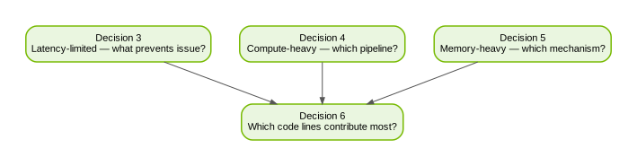
Primary check	Look for
Few source lines dominate the stalls, excessive wavefronts/requests/sectors, or instructions executed. A single line contributing more than ~30% of total stall samples, excessive wavefronts/requests/sectors, or Instructions Executed is a clear primary target. Use Instructions Executed (rather than stalls) when the kernel is compute-bound.	Source Counters: Top 3–5 source lines by sample count for the dominant stall reason, excess-transaction metric, or Instructions Executed from previous decisions. PM Sampling: Function Stats tool window
A single stall reason dominates a specific source line. Indicating a focused root cause.	Source Counters: Flag lines where one stall reason accounts for more than ~50% of that line’s total stall samples. PM Sampling: Function Stats tool window
Individual instructions show access-pattern problems localized to specific SASS locations.	Source Counters: SASS-level instructions where actual sector or wavefront counts exceed ideal counts by more than ~2×.
When tracking a hotspot across optimization iterations, absolute stall sample counts can change while the relative percentage value stays flat (or vice versa). Use absolute counts as the primary tracking signal. A percentage drop alone may just mean another line got worse.	Source Counters: Per-line stall sample counts and percentages, compared between baseline and optimized reports.
Warp convergence on the top-contributing source line is worse than the workload-wide average. The workload-wide convergence reported on the details page averages over all instructions. A specific hot line can be far below the average — costly if the line is also a major contributor.	Source Counters: Avg. Predicated-On Threads Executed for the hot source line; compare with the workload-wide value on the details page.
Samples may aggregate on a shared helper function This can include device-runtime helpers and templated math wrappers. When called from many sites, it can mask which call site is actually expensive.	Source page: Use the Inline Functions Table to attribute samples back to the calling source line. For large codebases, check aggregated metrics per file/per function first before drilling into individual lines.

Next Actions:

These actions apply to the decision as a whole, not to any individual primary check above.

• Hotspot identified: change one mechanism at a time (indexing, tiling, instruction mix, synchronization pattern).

• Change applied: re-profile and return to Decision 2: Is this latency-limited or throughput-limited?.

• Single kernel mixes different behaviors: split into separate kernels and re-evaluate each branch with this tree.

3.2.9. Decision 7: Are you close to hardware limits for this algorithm?

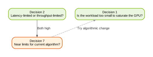
Primary check	Look for
Profiler observations align with the resource you expected to be busy. Compute SOL and memory SOL can both be high simultaneously with both inefficient compute and inefficient memory ops contributing. Confirm the chosen limiter is real: if you expect memory-boundedness, the memory-throughput metrics should be the ones near peak. If you expect compute-boundedness, a specific pipeline should saturate.	GPU Speed Of Light Throughput: gpu__compute_memory_throughput.avg.pct_of_peak_sustained_elapsed dram__bytes.sum.per_second
The limiter resource is within ~80% of its peak. Any unit can be the limiter — DRAM, L2, L1TEX, a specific compute pipeline, or scheduler issue rate. Confirm via the GPU Throughput Breakdown that the unit you identified in Decisions 4/5 is actually the dominant tier.	GPU Speed Of Light Throughput: GPU Throughput Breakdown
SM-level or warp-level load imbalance limits scaling even when the average case is fully optimized.	GPU and Memory Workload Distribution: sm__cycles_active.max / sm__cycles_active.avg — above ~1.2 indicates SM-level imbalance [6]. smsp__cycles_active.max / smsp__cycles_active.avg — flags warp-level imbalance.

[6]

The WorkloadImbalance rule fires at lower raw distance-from-average values (~5%) because it weights by the ratio of active to elapsed cycles.

Note

If the kernel being validated here was collected under different clock/cache/replay settings than the original triage pass, throughput ratios may not be directly comparable. Revisit Decision 0: Are the collected metrics trustworthy? to confirm collection consistency before declaring convergence.

Stop criteria:

• bottleneck is near architectural limits for the current algorithm, so stop micro-optimizing this implementation path and evaluate algorithmic changes (reformulation, decomposition, or tuned library substitution)

• high metric values contradict your expectation if the dominant limiter

• or next candidate change has low expected ROI relative to effort/risk for this algorithm, so return to workload-level diagnosis and choose a different algorithmic strategy

• or replacing a custom phase with a tuned library path already reaches target performance for this workload

If the above applies, return to Decision 1: Is the workload too small to saturate the GPU? and continue triage with the new algorithmic approach.

Note

Re-evaluate previously “converged” kernels on each new GPU architecture. Cache sizes, SM counts, register-file sizes, peak FLOPs, and feature support shift the dominant bottleneck. A kernel that was at architectural limits on one generation may have substantial headroom on the next, and previous optimization choices may now be the limiter.

On Blackwell (and later) the bytes-in-flight required to saturate DRAM per SM is substantially higher than on Ampere/Hopper because bandwidth has grown faster than SM count. A kernel that was DRAM-bandwidth-bound on A100 may become wavefront-bound or in-flight-bytes-bound on B200 and require more ILP, vectorized loads, or async copy. See Symptom: DRAM throughput is below peak with no other limiter saturated.

3.3. Timing and Collection Validity

Entry from workflow:

• Triage Workflow -> Decision 0: Are the collected metrics trustworthy? when metric trustworthiness is uncertain.

Note

• If full-section profiling is too slow, reduce workload size temporarily for iteration.

• Restore representative workload before final conclusions.

• Keep the profiling configuration identical between compared runs unless intentionally testing a control variable.

Note

• Timing trends remain consistent across repeated captures.

• Dominant bottleneck classification does not change when reducing metric set.

• Conclusions hold under both default and comparison control settings.

3.3.1. Symptom: Nsight Compute time differs from Nsight Systems

Common causes:

• Different timestamp methods between tools.

• NCU default clock locking (boost clock) vs. NSYS default behavior (no clock locking).

• NCU default cache handling vs. application cache state.

• NCU serialization/replay effects for multi-pass collection.

• Different clock domains drifting or changing across captures.

Actions:

• For cross-tool comparisons, test NCU with --clock-control none.

• Use --replay-mode application (or range replay) when cache priming matters.

• Use --cache-control none when you need application-managed cache state.

• Compare using the same workload scope and synchronization boundaries.

• Track relevant domain clocks (SM/L2/DRAM) and compare runs only under equivalent frequency behavior.

3.3.2. Symptom: Metric values are outside expected ranges

Common causes:

• Multi-pass mismatch on short or variable workloads.

• Tiny kernels that do not saturate units.

• Asynchronous engines contributing traffic to shared resources.

Actions:

• Increase workload duration and GPU saturation.

• Collect fewer metrics per run to reduce replay complexity.

• Prefer metrics known to share clock domain and collection pass when possible.

3.3.3. Symptom: Profiling overhead changes process time

Interpretation:

• Kernel execution time metric can remain stable while process runtime increases.

• More counters can increase pre-launch/post-processing overhead and replay count.

• In PM Sampling timeline rows, queue wait/idle phases can dominate wall-time without changing kernel-internal bottlenecks.

Actions:

• Start with smaller section sets, then add targeted metrics.

• Avoid heavy SASS patching metrics unless needed for root-cause analysis.

• If available, inspect PM Sampling timeline rows for queue wait/idle and semaphore wait signals to separate orchestration gaps from kernel inefficiency.

• If timeline gaps appear between dispatch-start and block-launch style rows, prioritize launch/orchestration investigation before kernel micro-optimization.

• Collecting a full metric set replays each kernel many times. Restrict --kernel-name (or equivalent filters) to a representative launch when iterating, and profile a single instance of repeated kernels by name rather than all of them.

3.3.4. Symptom: Optimization decisions don’t generalize across inputs or iterations

Common causes:

• Data-dependent kernels (e.g. neighbor lists, sparse operators) take very different paths and times across realistic inputs.

• Iterative algorithms exhibit different per-iteration behavior (e.g. progressive reduction shrinks the work set, sparsity patterns evolve).

• Templated kernels and multi-step schemes instantiate into multiple distinct kernels with different bottlenecks.

Actions:

• Profile with realistic, varied inputs — an optimization that helps one input can hurt another.

• Capture all kernel launches of an iterative algorithm in a single session so per-iteration behavior is visible.

• Profile each template instantiation and each step type separately rather than averaging across them.

• Re-run the dominant launch through this triage tree before assuming a fix generalizes.

3.3.5. Symptom: Nsight Compute PM Sampling shows dispatch/queue gaps

Interpretation:

• Range-level dispatch orchestration can be the primary limiter even when individual kernels look healthy.

• Queue wait/idle and semaphore stalls indicate command/synchronization pacing issues between kernels in the profiled range.

Actions:

• When profiling a range, compare dispatch-start, block-launch, and active-compute timeline rows to locate idle windows.

• Reduce unnecessary synchronization scope and tighten dependency chains.

• Increase dispatch batching/submission cadence when launch gaps dominate.

• Re-profile and return to Decision 2: Is this latency-limited or throughput-limited? before deeper kernel-level tuning.

3.4. Compute Pipeline Throughput

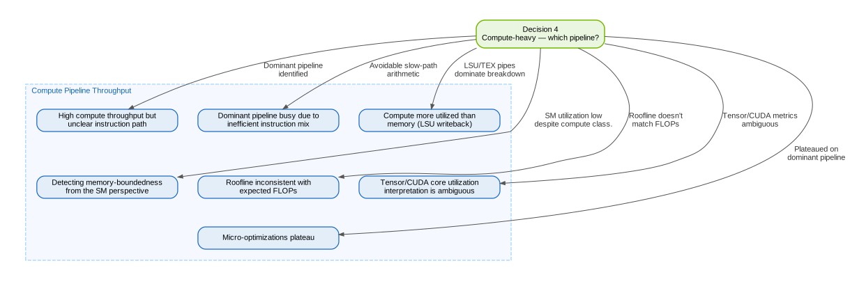
Entry from workflow:

• Triage Workflow -> Decision 4: If compute-heavy, which pipeline is the limiter? for compute-heavy branches.

Note

General optimization guidance

• Increase instruction-level parallelism (ILP) to hide dependent latency.

• Mix independent work so schedulers can issue every cycle.

• Avoid drawing conclusions from a single top-line throughput percentage.

Note

Pipeline metric names vary across compute capabilities. For example, sm__pipe_fma_cycles_active exists on SM 7.0–8.0, while SM > 8.0 splits it into fmalite and fmaheavy; sm__pipe_tensor_cycles_active applies to SM 7.0–12.0, while SM 10.x+ adds sm__pipe_tc_cycles_active for UTCMMA-capable chips. Other pipe names (fp16, fp64, alu, xu) also shift between architectures. Run ncu --query-metrics | grep sm__pipe_ on your target GPU to discover the available pipeline metrics before writing analysis scripts or setting thresholds.

3.4.1. Symptom: High compute throughput but unclear instruction path

Interpretation:

• SM Throughput is computed as the max over several sub-metrics.

• You must inspect the compute throughput breakdown to identify the true limiting pipeline (see Metrics Structure).

• High top-line throughput can still hide low utilization in other pipelines; optimize the dominant breakdown contributor first.

Actions:

• Open the throughput breakdown and identify the highest contributing pipeline.

• After identifying the dominant pipeline, drill into the source page and rank lines by Instructions Executed (filtered by that pipeline if filtering is available) to find the lines responsible for the bulk of work on that pipe.

• Verify instruction mix in Instruction Statistics.

• For tensor workloads, use sm__ops_* metrics to break down datatype/path/sparsity (metric components and pipeline names are documented in Metrics Decoder).

• Keep active-vs-elapsed semantics consistent when comparing before/after runs (see Metrics Structure).

3.4.2. Symptom: Dominant pipeline is busy due to inefficient instruction mix

Actions:

• Identify expensive instruction classes in the dominant pipeline (e.g. FP64 or unfused sequences).

• Prefer fused/equivalent lower-cost instruction forms when numerically acceptable.

• Re-profile pipeline-specific utilization and total kernel duration after each change.

3.4.3. Symptom: Compute is more utilized than memory

Interpretation:

• The top compute pipeline may be limiting progress even if memory is active.

• High LSU contribution can indicate instruction-side pressure from memory operations: the bottleneck may be the SM/Compute resources that issue memory instructions and kick off the transactions, which is distinct from the memory subsystems that fulfill them. Fixing the latter does nothing if the former is the limiter.

LSU writeback disambiguation:

When L1TEX LSU writeback (data return from L1 to SM) is high, two distinct scenarios exist and require different responses:

• Low instruction throughput + high LSU writeback: the writeback path is saturated by wide loads (64-bit or wider per thread). Each load occupies the writeback bus for multiple cycles, limiting the rate at which results return to the SM. Optimization: reduce data width per load (e.g., use float instead of double where precision allows) or restructure the algorithm to reduce the number of wide loads per warp.

• High instruction throughput + high LSU writeback: the SM is issuing many memory instructions at high rate and the writeback path is saturated by sheer volume even with narrow loads. Optimization: reduce total memory instruction count (improve data reuse, use shared memory, or cache in registers).

Actions:

• Inspect Compute Workload Analysis to identify dominant pipe(s).

• Correlate dominant pipe with Source hotspots and stall reasons.

• When LSU/TEX pipes dominate, check the LSU writeback and TEX writeback (tex2sm) SOL indicators to determine whether the data return path — not just the request path — is the true bottleneck.

• Remove redundant computation or phase coupling where possible.

3.4.4. Symptom: Memory-bound from the SM perspective

When SM utilization is low (low pipeline SOL), it is important to determine whether memory latency is the cause before pursuing compute-side optimizations:

• When SM utilization is low and memory indicators are also low, the kernel is likely latency-bound with insufficient ILP or occupancy; follow the stall/occupancy path (Decision 3: If latency-limited, what prevents instructions from issuing?).

• Check L1TEX throughput (data-stage and F-stage SOL). If L1TEX is high while SM pipes are low, the shader is memory-bound at the L1 level.

• Check L2 sector traffic from L1TEX (lts__t_sectors_srcunit_tex). If L2 traffic from L1TEX is high, the shader is missing in L1 and bound on L2 or DRAM.

• When both L1TEX and L2-from-L1TEX are high, the kernel is deeply memory-bound; follow the memory triage path (Decision 5: If memory-heavy, which memory mechanism dominates?) rather than attempting compute-side optimization.

3.4.5. Symptom: Roofline appears inconsistent with expected FLOPs

Common causes:

• Wrong roofline section for instruction type (e.g. FP32 roofline with tensor kernels).

• Measured clock basis differs from theoretical boost-clock assumptions.

• Model FLOPs and hardware FLOPs differ due to matrix shape expansion/padding.

Actions:

• Enable the correct roofline section for your data path (including tensor roofline).

• Cross-check reported SM frequency used by the profiler.

• Use operation counters and kernel/SASS inspection to validate true executed math.

• The hierarchical roofline overlays separate L1, L2, and DRAM ceilings on the bandwidth axis. When a kernel sits at the DRAM roof, cache efficiency is limiting throughput. Improving reuse can lift the achieved point above the DRAM roof and toward the L2 or L1 ceiling without changing arithmetic intensity.

3.4.6. Symptom: Tensor/CUDA core utilization interpretation is ambiguous

Interpretation:

• Tensor kernels typically show low scheduler issue-active but very high pipeline throughput per issued instruction. Each tensor instruction performs orders of magnitude more work than a scalar instruction, so a low issue rate is expected and not a sign of starvation.

• The IssueSlotUtilization rule scales its speedup estimate down in this regime; treat HighPipeUtilization (tensor pipe) as the primary signal instead.

Note

MMA fundamentals:

• Every Matrix Multiply-Accumulate (MMA) instruction computes D = A * B + C over an (M, N, K) tile, with approximately 2 * M * N * K FLOPs (one multiply and one add per inner element). C and D may alias to enable accumulation across multiple multiplications.

• A and B can use a different input format than C and D (e.g. FP16/BF16 inputs with FP32 accumulation), trading input bandwidth and storage for accuracy.

• Supported (M, N, K) shapes are architecture-, datatype-, and instruction-specific; consult the PTX manual for the target GPU.

• If the workload’s matrix size doesn’t match a hardware-supported MMA shape, tiling is required and produces wasted FLOPs at the boundary (compute outside the desired output region).

• Larger MMA tile shapes (e.g. 256×256×32 vs 16×8×8) deliver higher peak throughput but waste more work on small or non-square problems. For small or irregular matrices, prefer smaller MMA tile shapes to minimize wasted-work overhead. The optimal tile depends on matrix dimensions and alignment.

MMA families and how they appear in counters:

• Warp-level MMA (Volta+): runs on a single warp scheduler using all 32 threads of one warp. All inputs and outputs reside in the register file. Cannot be predicated — all 32 threads must be active, so divergent or early-exited lanes prevent issue. Source counters: 1 warp instruction with 32 threads predicated on average (cannot be lower).

• Warp-group MMA / WGMMA / GMMA (Hopper+): coordinates all four warp schedulers in the SM. Requires a block of at least 4 warps so one runs on each scheduler. Operand tiles are loaded directly from shared memory (effectively quadrupling the available register file), and a quarter of the output is written to each warp scheduler’s register file. Executes asynchronously: issue, do other work, then wait. Source counters show 4 warp instructions executed per logical MMA (one per participating scheduler) — divide by 4 when reasoning about logical operations issued. WGMMA acts like a barrier across the four schedulers. WGMMA acts like a barrier across the four schedulers. A late-arriving warp causes the others to stall as warpgroup_arrive (see Symptom: Warp stall breakdown dominated by specific stall reasons).

• 5th-generation MMA (Blackwell): adds a tensor-core controller pipeline shared by the four warp schedulers and a separate on-chip Tensor Memory (TMEM) that holds operands/outputs, removing register-file pressure. A can come from shared memory or TMEM, B from shared memory, D is written to TMEM. Issued by a single thread of a single warp; counters show 1 warp instruction with 1 active thread per issue while the controller drives all four schedulers — this is expected, not warp starvation. Two-CTA variants (CUDA clusters) allow matrices to span two SMs. TMEM must be explicitly allocated, relinquished (so other warps on the SM can reuse it), and deallocated before kernel exit. Failure to deallocate leaks memory and can cause CUDA errors.

Pipelining and warp specialization:

• TMA copies are issued by a single thread and free warps from address-math work, which itself can dominate a kernel. Pipeline TMA loads with async MMA (issue next tile’s TMA while current tile’s MMA executes, then ping-pong) to hide memory latency.

• Async MMA + async TMA only pay off if the kernel actually overlaps them; ensure waits are placed late enough to allow overlap, otherwise the kernel collapses to the synchronous “load → compute → load” pattern.

• Warp specialization dedicates some warps to data movement (TMA loads) and others to compute (MMAs), enabling deeper pipelines and better overlap of memory and math.

Understanding utilization:

• Tensor pipeline utilization over time is the key signal that the tensor cores are actually being kept busy.

• Cross-check expected vs. actual TMA bytes in/out, shared-memory request count, and TMEM traffic against the algorithm’s tile sizes to confirm the kernel is doing what was intended. Replacing a register-file operand load with a TMEM load (5th-gen) reduces shared-memory request count for that operand and shifts traffic to TMEM equivalents — verify that shift is visible.

• Computing global-to-shared address indexing for tiles is often a real bottleneck and can dominate over the MMA math itself. If address-math pipelines (e.g. ADU) saturate before the tensor pipe, offload indexing to TMA.

Actions:

• Treat throughput metrics as pipeline utilization, not marketing-core counts.

• Map workload instructions to their physical/logical execution pipelines (see Streaming Multiprocessor model and Metrics Decoder).

• Confirm whether instructions are fixed-latency math, variable-latency memory, or queue-limited tensor operations.

• Choose the largest MMA shape that still fits the problem to reduce per-instruction issue overhead, but switch to smaller shapes when the problem is not a multiple of the tile and wasted-work would dominate.

• For sparse-tolerant inputs, consider sparse MMA variants — they exploit a fixed structured-zero encoding to halve input/output data, effectively doubling effective bandwidth and throughput when the data fits the sparsity pattern.

3.4.7. Symptom: Micro-optimizations plateau

Consider algorithmic changes:

• Split mixed-behavior kernels into phase-specific kernels.

• Offload dense linear algebra phases to tuned libraries when equivalent.

• For tensor-core kernels, CUTLASS, CuTe, and the CuTe DSL abstract MMA shape, datatype, and pipelining for the target hardware. Using them is often a faster path to peak throughput than hand-tuning warp-group or 5th-gen MMA pipelines (see Symptom: Tensor/CUDA core utilization interpretation is ambiguous).

• Re-assess end-to-end runtime, not just individual kernel percentages.

3.5. Memory Access Patterns and Transaction Efficiency

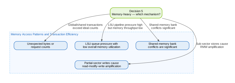
Entry from workflow:

• Triage Workflow -> Decision 5: If memory-heavy, which memory mechanism dominates? for access-pattern and transaction-efficiency issues.

Note

Memory analysis fundamentals:

• Memory is organized into 128-byte cache lines, each split into four 32-byte sectors (typically eight 4-byte elements per sector).

• At the warp level, load instructions are packaged into wavefronts: groups of parallel accesses that the memory subsystem can service in one step.

• With perfect coalescing, a warp’s loads form a single wavefront.

• L1 has a tag stage and a data stage, each producing wavefronts based on the access pattern.

• Tag-stage wavefronts ≈ distinct cache lines touched by the warp (32 threads spanning N cache lines → roughly N/4 tag wavefronts).

• Data-stage wavefronts depend on the intra-cache-line sector pattern: 32 threads spread across the four sectors of four cache lines = 1 data wavefront, but 32 threads clustered on one sector per cache line = 4 data wavefronts.

• The same number of cache lines touched can produce very different data-stage counts.

• Shared memory is organized as 32 banks of 4-byte cells; each bank serves one 4-byte cell per cycle. A full row across all 32 banks is 128 bytes, matching the L1 cache line size.

3.5.1. Symptom: Unexpected bytes or request counts

Common causes:

• Strided writes causing many more sectors/wavefronts than expected.

• Partial-sector writes increasing traffic overhead.

• L2 serving as coherence point (device-memory writes may not immediately appear at DRAM).

Actions:

• Inspect access pattern per instruction (coalesced vs. strided).

• Quantify request bytes and return bytes per instruction.

• Distinguish tag lookups, fill traffic, write-through, and eviction traffic.

• Use Memory Tables columns explicitly: Instructions -> Requests -> Wavefronts -> Sectors to identify where inflation starts.

• Prefer structure-of-arrays over array-of-structure when warp threads each touch a single field. The former usually restores coalescing because consecutive threads read consecutive addresses of the same field.

• When comparing per-instruction inefficiency across hot lines, normalize transaction counts by the number of times the instruction executed. Frequently-executed instructions otherwise dominate naively even when their per-execution efficiency is fine. The cost of an inefficient pattern only matters in proportion to how often it runs.

• Vectorize loads (e.g. float4) when alignment permits: a single instruction fetches multiple cache lines and exposes more bytes in flight per issue, using a dedicated SASS fast path. Vectorization on regular layouts (e.g. structured stencils) does not have the alignment problems that block TMA on irregular kernels.

• For halo-style access (stencils, local-window kernels), use vector loads on the contiguous interior and scalar loads on the halo tail, where neighbors are individual elements.

• Tile so each thread computes a small N-D output region: load each input once, then distribute its contribution to all output partial sums it affects. This converts redundant halo loads into reuse and can shift a kernel from L1-wavefront-bound to DRAM-bandwidth-bound.

3.5.2. Symptom: LSU queue pressure with low overall memory utilization

Interpretation:

• Frequent local/global instructions can stall on LSU queue availability.

• This often indicates transaction inefficiency, not raw bandwidth saturation.

• A single request can require multiple wavefronts, so high wavefront pressure may be a pipeline-serialization issue even when sectors/request is moderate (see Metrics Quantities).

• Wavefront pressure (data-pipe LSU wavefronts) is increasingly the limiter on Blackwell because the memory subsystem rate scales with SM count while DRAM bandwidth has grown faster than SM count. Increasing L1 bandwidth alone does not fix wavefront pressure: it is a rate/instruction issue, not a bandwidth issue.

Actions:

• Inspect Warp State for LG/LSU throttle style stall reasons. lg_throttle indicates the L1 instruction queue is full and is a clear signal of L1 pressure.

• In Source page, compare ideal and actual global transactions per line.

• Prioritize refactors on lines with largest inefficiency ratio.

• Re-check memory throughput after improving transaction efficiency.

• Check Sectors/Req and Wavefronts in Memory Tables to decide whether to prioritize coalescing or reducing internal L1TEX wavefront serialization first.

• When data-pipe LSU wavefront utilization is high but DRAM throughput is sub-peak, the kernel is wavefront-bound, not bandwidth-bound. Adding more in-flight loads (see Symptom: DRAM throughput is below peak with no other limiter saturated) will not help. Change the access pattern instead: vectorize, tile, reorganize threads, or use sub-warp / row-data parallelism. Cooperative threads in a sub-warp can use __shfl_sync to share partial results via registers without going through shared memory.

3.5.3. Symptom: Shared-memory bank conflicts are significant

Interpretation:

• Wavefronts per request equals the max number of distinct cells any single bank must serve. The request takes that many cycles. Bank conflicts equal the number of wavefronts - 1.

• A 4-byte-stride access (thread i reads bank i) is the ideal case: 1 wavefront, 0 conflicts.

• Random shared-memory access is not automatically bad: as long as each bank serves a single thread, the request still completes in 1 cycle.

• Broadcast (multiple threads reading the same address) is conflict-free — the bank broadcasts the value to all requesters in 1 cycle.

• The pathological case is stride = 128 bytes: all 32 threads land on the same bank, producing 32 wavefronts and 31 conflicts.

• ideal wavefronts > 1 when per-thread access width exceeds 4 bytes (e.g. double requires at least 2 wavefronts per warp even with no conflicts).

• Per-instruction bank-conflict counts in the source view can be lower than the aggregate counts in the memory tables, because the tables also include cross-client conflicts between shared-memory and L1 accesses targeting the same physical banks in the same cycle.

• Shared memory and L1 favor different access patterns: a stride that is conflict-free for shared (e.g. diagonal) can be costly for L1 (many cache lines), and vice versa.

• Worst-case sanity check: for N shared-memory requests, the absolute worst case is 32 × N bank conflicts (every thread of every request landing on the same bank). Use this to sanity-check whether observed conflict counts are close to the pathological ceiling.

• Bank conflicts typically correlate with short_scoreboard stalls on the consuming instruction. If bank conflicts are the real bottleneck, short_scoreboard is usually high — but the converse does not hold (high short_scoreboard has other causes too; see Symptom: Warp stall breakdown dominated by specific stall reasons).

Actions:

• Confirm bank-conflict intensity in memory tables and source-correlated counters.

• Remap shared-memory indices/padding so threads in a warp map to distinct banks.

• Re-profile and confirm both bank conflicts and kernel duration improve.

3.5.4. Symptom: Partial-sector writes cause read-modify-write amplification

Interpretation:

• Stores that write fewer bytes than a full sector (32 bytes) force the memory subsystem to read the existing sector, merge in the new bytes, and write it back.

• This read-modify-write overhead can silently double effective bandwidth for write-heavy kernels.

• Common sources: byte-granularity stores (e.g. char or short outputs), strided stores that leave gaps within a sector, and structure-of-arrays with narrow fields.

Actions:

• Widen store granularity: pack narrow outputs into wider types (e.g. int or float4) or use vectorized stores to fill full sectors.

• Align stores so that consecutive threads in a warp write consecutive sector-aligned addresses.

• Check Sectors/Req in Memory Tables for sector fragmentation.

• Re-profile write bandwidth and kernel duration after alignment improvements.

3.6. Memory Subsystem and Bandwidth Bottlenecks

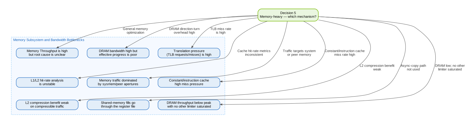
Entry from workflow:

• Triage Workflow -> Decision 5: If memory-heavy, which memory mechanism dominates? for memory-heavy branches.

Note

General optimization guidance

• Prioritize coalescing and sector reuse before policy tuning.

• Test persistent/evict policy only when dataset and reuse pattern justify it.

• Validate improvements by checking both bandwidth metrics and kernel duration.

• Treat L1/TEX, shared memory, L2, and compression as separate potential limiters. Memory Throughput is a roll-up and not a root cause by itself (see also Hardware Model memory hierarchy).

Note

For memory-dominated kernels:

• Estimate achieved bandwidth from moved bytes and kernel duration.

• Compare against a practical bandwidth baseline for the same platform.

• If close to practical peak and stalls are expected long-scoreboard waits, further gains may require algorithmic change, not micro-tuning.

Note

Use shared memory when:

• Data is reused multiple times by threads in the same block.

• Threads in a block must cooperate or synchronize on intermediate results.

• You want explicit, deterministic on-SM caching with predictable residency.

• The natural access pattern maps better to banks than to cache lines.

• Block-level reduction or pre-aggregation can replace global atomics or repeated global loads.

Note

L1 cache and shared memory share the same physical backing storage on the SM. A runtime carveout assigns part to shared memory and the remainder to L1. L1 hits and shared-memory loads therefore have similar latency and throughput, so the choice between them should be driven by access-pattern fit (banks vs cache lines). Larger shared allocations leave a smaller L1 cache — pick the carveout that matches the kernel’s reuse pattern.

3.6.1. Symptom: Memory Throughput is high but root cause is unclear

Interpretation:

• Memory Throughput is a max-over-subsystems metric.

• L1, L2, and DRAM can each be limited by different mechanisms.

• A profile showing ~90% Memory Throughput can be misleading: Expand the breakdown to see whether DRAM, L2, L1, or wavefronts (data-pipe LSU wavefront utilization) are the actual limiter. On Blackwell and later, wavefront pressure is increasingly the binding constraint before DRAM bandwidth is reached.

• Compare effective bandwidth (analytically useful bytes / time) against raw DRAM throughput. A large gap is overfetch — typically L2 thrashing forcing refetches from DRAM — and means the kernel is moving far more data than it logically needs. A high raw DRAM throughput with low effective bandwidth is not real efficiency.

Actions:

• Expand the memory throughput breakdown and identify the dominant unit.

• Prefer DRAM metrics in the memory-controller clock domain for DRAM saturation analysis.

• Use source/node filters for L2 counters when isolating SM traffic from non-SM engines.

• In the Memory Chart, check both link utilization and in-unit port utilization; links can be moderate while a shared port is already saturated.

• When PCIe traffic overlaps kernels, inspect read/write directions separately; PCIe is full-duplex while DRAM paths are effectively half-duplex at the memory protocol level.

• High L1 hit rate combined with a high L2 hit rate on the same data indicates the data is re-read repeatedly through the cache hierarchy — staging into shared memory could reduce cache pressure and free L1 capacity for less reusable data.

Note

lts__t_sectors_lookup_miss.sum is not equivalent to dram__sectors.sum. L2 misses can generate both fill sectors and eviction write-back sectors (if the evicted line is dirty), and writes (hit or miss) may generate write-through sectors to DRAM. Always use dram__sectors directly when quantifying actual DRAM traffic.

Note

DRAM write bytes can be significantly lower than total global store bytes because the GPU L2 cache is the point of coherence for device memory. Stores that hit in L2 may never propagate to DRAM; eviction to device memory occurs only when the L2 needs the cache line for other data. Do not assume a 1:1 relationship between STG instructions and DRAM write traffic.

3.6.2. Symptom: DRAM throughput is below peak with no other limiter saturated

Interpretation:

• Average bytes in flight ≈ achievable bandwidth × memory latency (Little’s Law). Saturating the memory bus requires keeping enough requests outstanding for that chip.

• Modern GPUs require many more in-flight bytes per SM than older ones because bandwidth has grown faster than SM count. A kernel that saturated the bus on A100 (~2 TB/s) may fall well short on B200 without modification, because each SM must now issue more requests.

• With insufficient in-flight requests, the bus is starved even when access patterns are coalesced and caches behave well.

• Performance vs. bytes-in-flight follows a roofline-like curve: below a transition point, bandwidth is limited by lack of requests. Above it, the kernel can reach close to peak.

• Bytes in flight cannot be read directly from a single counter. It is inferred when DRAM is low and nothing else is saturated.

• Two primary tools keep the bus saturated: maximize warps resident per SM (occupancy) and issue more independent loads per warp (ILP).

Diagnostic signals:

• gpu__dram_throughput.avg.pct_of_peak_sustained_elapsed well below peak.

• No SM pipeline (sm__pipe_*_cycles_active) near saturation.

• l1tex__data_pipe_lsu_wavefronts.avg.pct_of_peak_sustained_elapsed not near peak (rules out wavefront-bound — see Symptom: LSU queue pressure with low overall memory utilization).

• High long_scoreboard stalls without coalescing inefficiency (sectors-per-request near ideal, bytes-per-sector near 32).

Actions:

• Raise occupancy so the SM has more eligible warps to issue from when others stall on memory; see Symptom: Low utilization despite acceptable occupancy.

• Add ILP via unrolling: each thread processes K elements, all loaded before any are consumed. This trades registers for additional concurrent independent loads. Unrolling can also reduce L2 thrashing by changing the temporal ordering of accesses so threads in a warp issue many high-locality loads close together.

• Vectorize loads (e.g. 16-byte loads with proper alignment). They use a dedicated SASS fast path and produce more bytes in flight per issued instruction.

• Issue loads early, consume late: spacing dependent uses away from their producing loads lets a warp issue many requests before stalling on a data dependency. Issuing dependent instructions immediately after a load forces an immediate stall.

• When register or shared-memory pressure caps these techniques, switch to async copies (see Symptom: Shared-memory fills go through the register file) or L2 prefetch. They stage data without consuming registers.

• Sweep tunable parameters (unroll factor, K elements per thread, cooperative group size). The sweet spot is workload- and architecture-dependent. The same factor that wins on Hopper may not win on Blackwell.

Stop criteria:

• If DRAM throughput is now near peak, the kernel has crossed the saturation knee. Remaining gains require algorithmic redesign (less data, better reuse), not more in-flight requests.

• If wavefront utilization rises but DRAM stays sub-peak, the limiter has shifted to wavefronts — follow Symptom: LSU queue pressure with low overall memory utilization.

3.6.3. Symptom: Shared-memory fills go through the register file

Interpretation:

• The traditional path to shared memory is Device → L2 → L1 → register file → shared memory, which costs two instructions per element and consumes register-file bandwidth.

• On Ampere and newer, cp.async / LDGSTS moves data directly from global memory through L1 into shared memory in a single instruction, avoiding register-file pressure. cp.async is element-wise and not as fully asynchronous as TMA — subsequent loads can interfere and prevent the desired overlap.

• An alternate async-copy path bypasses L1 storage entirely; prefer it when the data is not also needed via L1.

• If the kernel has a producer-loop that loads then stores into shared memory, but the memory chart still shows traffic on the register-file path, the async-copy path is not actually being exercised.

Hopper+ adds two more asynchronous staging tools that complement cp.async:

• TMA (Tensor Memory Accelerator): a dedicated SM engine that performs single-threaded DMA copies from global memory through L2 directly into shared memory, asynchronously, with a separate engine. TMA triggers transfers that can overlap with concurrent regular loads. TMA can also perform swizzling and transposition during the copy, eliminating separate shared-memory rearrangement passes. Strict alignment requirements (16-byte global, 16-byte stride multiple, 128-byte aligned shared, 16-byte transfer size, block dim ≤ 256 elements) can make TMA an obstacle for irregular-pattern kernels (e.g. SpMV) but a natural fit for dense tiled kernels.

• L2 prefetch (inline PTX): warms the L2 cache without using shared memory and without requiring explicit synchronization. Alignment is easy (read a little before/after the target region). This is often the easiest async tool to adopt when the shared-memory budget is already tight.

Pipelining is important:

• A synchronous pattern (load tile → wait → compute → wait → load next tile) leaves async tools idle and underperforms.

• Issue several stages of TMA loads up front, then in steady state overlap stage-i compute with stage-(i+1) load. Hold num_stages tiles in shared memory and march through the slow direction, reissuing TMA into a slot once its compute is complete.

• Pipelined TMA needs __syncthreads to ensure all threads finish using a shared-memory slice, plus a fence.proxy.async to order generic-proxy SM accesses before subsequent async-proxy TMA operations. Use a parity bit on mbarrier.try_wait.parity to reuse the same barrier across iterations.

Actions:

• In the Memory Chart and Memory Tables, inspect per-path traffic to confirm which path is carrying the shared-memory fill.

• Convert the global-load-then-shared-store sequence to cp.async (or use libraries that emit it, e.g. CUTLASS).

• If L1 caching of the same data is not needed, prefer the L1-bypassing async-copy variant.

• Choose the lightest tool that fits the access pattern: cp.async for element-wise patterns, TMA for dense aligned tiles where swizzle/transpose would otherwise cost extra passes, and L2 prefetch when shared memory is the binding resource or the access pattern is too irregular for TMA’s alignment rules.

• For TMA-staged kernels, ensure waits are placed late enough to allow overlap. Itherwise, the kernel collapses to the synchronous pattern.

• Re-profile to confirm reduced register-file activity, fewer issued memory instructions, and shorter kernel duration.

3.6.4. Symptom: L1/L2 hit-rate analysis is unstable

Common causes:

• Hit and miss counters captured in different replay passes.

• Cache state variation between passes (primed vs. flushed).

• Workload too short to provide stable ratios.

Actions:

• Increase workload duration.

• Reduce metrics to encourage same-pass collection for related counters.

• Control replay/cache settings and keep them constant across comparisons.

3.6.5. Symptom: Memory traffic is dominated by sysmem/peer apertures

Interpretation:

• Kernel memory pressure may come from data placement, not only coalescing/cache efficiency.

• SysL2 aperture-heavy traffic often has higher latency than local device-memory paths.

Actions:

• Split memory traffic by destination aperture (device vs sysmem vs peermem) when metrics are available.

• Verify aperture metrics to confirm requests are hitting peer/system memory paths.

• Move hot, repeatedly accessed data to local device memory and stage ingress/egress explicitly.

• Re-profile to confirm reduced aperture traffic and lower memory-latency stalls.

3.6.6. Symptom: Constant/instruction cache hierarchy has high miss pressure

Interpretation:

• Kernels can be limited by constant or instruction fetch behavior, not only data-path bandwidth.

• GCC/constant/instruction cache miss traffic can surface as latency stalls with moderate DRAM utilization.

Actions:

• Inspect constant and instruction cache hit-rate trends across hierarchy levels.

• Reduce instruction-footprint churn and excessive constant-data working-set pressure.

• Re-profile to confirm reduced miss-path traffic and improved issue efficiency.

3.6.7. Symptom: L2 compression benefit is weak on compressible traffic

Actions:

• Inspect write/update patterns for irregularity that defeats compression.

• Improve locality and write regularity for data expected to compress well.

• Re-check compression-related counters and effective bandwidth.

3.7. Memory Contention and Synchronization Overhead

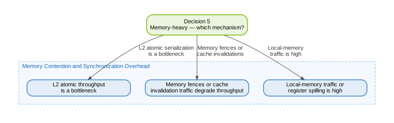
Entry from workflow:

• Triage Workflow -> Decision 5: If memory-heavy, which memory mechanism dominates? for contention and synchronization-related memory bottlenecks.

3.7.1. Symptom: L2 atomic throughput is a bottleneck

Interpretation:

• Global atomics (atomicAdd, atomicCAS, etc.) are serialized at the L2 atomic stage.

• When many warps contend on the same or nearby addresses, L2 atomic throughput becomes the limiter.

• This often manifests as moderate L2 throughput with high long-scoreboard stalls, because the SM is waiting for the atomic to complete.

• lts__t_requests_op_atom can confirm the volume; high atomic request rates relative to total L2 traffic indicate this bottleneck.

• Algorithms that progressively reduce into a shrinking set of accumulators (e.g. iterative merge / bucket-collapse reductions) get slower over time because atomic collisions increase as the target set shrinks.

• Issuing a global atomic from every thread of a very large grid (e.g. millions of threads) oversubscribes the memory pipeline regardless of collision count.

Actions (apply hierarchically — each level reduces the pressure on the next):

1. Warp level: combine values among threads of the same warp using shuffle-based reductions (__shfl_*_sync) or __reduce_*_sync. This collapses up to 32 atomics into 1 per warp.

2. Block level: if the reduction set fits in shared memory, finish the reduction there. Shared-memory atomics are served inside the SM and are significantly faster than global atomics. Emit at most one global atomic per block.

3. Privatization: for histogram-style patterns where target indices are scattered, build per-block (or per-warp) local histograms in shared memory and merge them in a final pass.

4. Re-profile L2 atomic request counters and kernel duration after each step; expect lg_throttle and drain stalls to drop together with atomic request volume.

3.7.2. Symptom: Memory fences or cache invalidation traffic degrade throughput

Interpretation:

• __threadfence(), __threadfence_block(), __threadfence_system(), and cooperative-group synchronization primitives enforce ordering by draining in-flight memory operations and/or invalidating caches.

• Frequent fences inject serialization latency that does not appear as a traditional stall reason but shows up as reduced issue efficiency and increased memory-system idle time.

• Cache invalidation traffic triggered by fences can also inflate L2 and DRAM bandwidth with non-productive requests.

• Cooperative-group grid.sync() and multi-grid synchronization can force full-device drain and invalidation cycles.

Actions:

• Audit fence frequency: ensure fences are used only at producer-consumer boundaries, not inside inner loops.

• Prefer __threadfence_block() over __threadfence() when inter-block ordering is not required; block-scope fences are cheaper.

• Minimize __threadfence_system() to cases that genuinely require CPU-visible ordering.

• If cooperative-group grid-level synchronization is frequent, consider restructuring into multiple kernel launches with implicit inter-kernel ordering instead.

• Re-profile issue efficiency and memory throughput after reducing fence scope or frequency.

3.7.3. Symptom: Local-memory traffic or register spilling is high

Interpretation:

• The Launch Statistics / Source page reports per-kernel stack frame size, spill stores, and spill loads. A non-zero stack frame means the compiler allocated local memory for register-pressure relief.

• Spills surface as L1/L2 traffic on local-memory paths and as long_scoreboard / lg_throttle stalls on the consumer instructions; they often look like a generic memory-bound symptom even when the algorithm fits in registers.

• A spilling kernel can be both occupancy-limited (registers per thread) and memory-bound (spill traffic) at the same time, so improvements may need to come from both directions.

Actions:

• Inspect the Source view for LDL / STL instructions to localize the spilling region. Also rank source lines by L2 Theoretical Sectors Local — the top contributors are the ones generating the most local-memory traffic.

• Reduce live-range overlap (split kernels, recompute cheap values, restructure inner loops) before forcing a register cap.

• Cap registers per thread (__launch_bounds__, -maxrregcount) and re-measure: if spills increase, the cap is too aggressive and is trading occupancy for spill traffic.

• Locate spill-heavy source/SASS lines and reduce live ranges or temporary arrays.

• Re-balance launch geometry only if it materially reduces spill-driven local traffic.

• Re-check local-memory counters (l1tex__t_sectors_pipe_lsu_mem_local_op_*) and end-to-end kernel duration.

3.8. Occupancy, Scheduling, and Stall Analysis

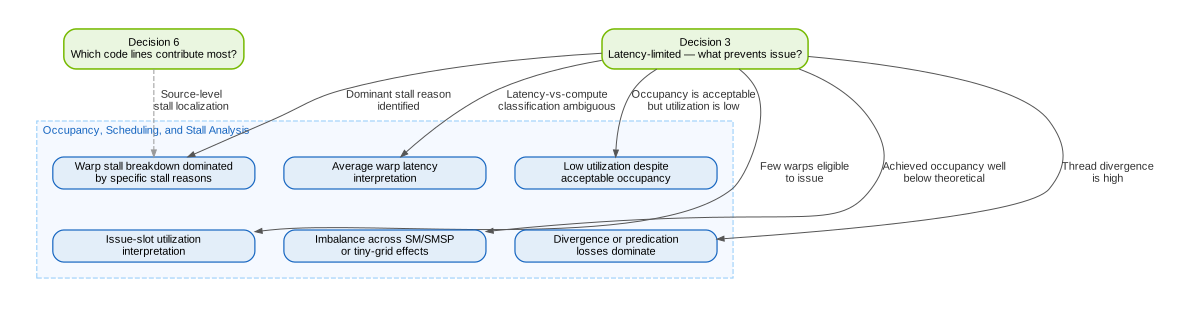
Entry from workflow:

• Triage Workflow -> Decision 3: If latency-limited, what prevents instructions from issuing? for latency/issue-efficiency limits.

• Triage Workflow -> Decision 6: Which code lines are the top contributors? for source-level stall localization follow-up.

Note

General optimization guidance

• Keep enough independent warps per scheduler to hide fixed and variable latency.

• Favor launch geometry that improves both active warps and issue-active cycles.

• Treat stall reduction as successful only when kernel duration also improves.

Note

When shared-memory sweep reduction dominates stalls:

• Consider two-stage warp-shuffle reductions to reduce shared-memory traffic.

• Keep synchronization minimal and verify correctness first.

• Re-profile to confirm stall shift and net duration gain.

3.8.1. Symptom: Low utilization despite acceptable occupancy

Interpretation:

• Higher occupancy alone does not guarantee speedup.

• If in-flight memory operations are insufficient, latency remains exposed.

Use the occupancy-vs-utilization quadrant to classify the situation:

• High occupancy + high utilization: SM or memory are saturated. Further occupancy gains are irrelevant; reduce algorithmic work or restructure the kernel.

• High occupancy + low utilization: warps are present but stalled — this is a latency-bound regime. Look at the top stall reason (and the full stall breakdown, not only long_scoreboard / barrier) to identify what is the blocking issue. Increasing occupancy further will not help: focus on latency hiding (ILP, prefetch, pipeline interleaving) instead.

• Low occupancy + high utilization: the active warps are keeping the SM (or the memory system) saturated despite few warps being resident. Adding more warps could compete for the already-saturated resource and may hurt performance. Optimize the hot pipeline or memory tier first (see Decision 4: If compute-heavy, which pipeline is the limiter? / Decision 5: If memory-heavy, which memory mechanism dominates?).

• Low occupancy + low utilization: both occupancy and useful work are low — this is either an underfill or a launch-limiting-resource issue. Determine whether the SM can accept more warps (check warp-can’t-launch classification below) and whether feeding more work would improve throughput.

When achieved occupancy is significantly below theoretical, identify the primary launch-limiting resource using launch__occupancy_limit_* metrics and the Occupancy Calculator:

• Register limited: the SM register file is fully allocated; an additional warp would exceed the register budget. Reduce registers per thread (--maxrregcount, __launch_bounds__) or reduce live variable ranges.

  Conversely, registers per thread can be increased without penalty as long as the larger count still falls within the same theoretical-occupancy bracket on the target GPU. Use the Occupancy Calculator to find the next quantization step; below that step, additional registers cost nothing in resident warps and can buy ILP, fewer reloads, or fewer spills. Only reduce registers when the kernel sits just above a quantization boundary or when the reduction would unblock a target occupancy.

• Shared-memory limited: the SM shared-memory partition is fully allocated. Reduce per-block shared-memory usage or reshape block dimensions.

• CTA-slot limited: maximum concurrent blocks per SM reached. Use smaller blocks or adjust maxThreadsPerBlock.

• Warp-slot limited: maximum concurrent warps per SM reached (e.g. large blocks can fill all warp slots with few blocks). Consider reducing block size.

Resource allocation quantization: occupancy is a step function of resource usage. When a kernel is near a quantization boundary (e.g., 33 registers per thread on a GPU where 32 would permit an extra warp slot), even a one-register reduction can produce a measurable occupancy jump. Use the Occupancy Calculator to identify these thresholds.

Actions:

• Compare occupancy with issue activity and warp stall breakdown.

• Check whether active warps are actually eligible to issue.

• Increase independent work per warp and/or per block before only tuning occupancy.

• Unrolling and vectorized loads are typically the first ILP techniques to try because they raise both the number of independent loads and bytes in flight. Their cost is register pressure, so re-check occupancy after the change. When the kernel is memory-latency-bound and DRAM is sub-peak, see Symptom: DRAM throughput is below peak with no other limiter saturated for the full bytes-in-flight background.

• Remember that warps are scheduled per SM sub-partition (SMSP); inspect scheduler-level metrics before applying SM-level conclusions (see Streaming Multiprocessor model).

• Check active-threads-per-warp style metrics to avoid mistaking divergence-heavy warps for healthy occupancy.

3.8.2. Symptom: Warp stall breakdown dominated by specific stall reasons

Each active-cycle, every warp reports exactly one smsp__warps_issue_stalled_* reason. selected means the warp issued an instruction; not_selected means it was eligible but the scheduler picked a different warp. All other reasons are true stalls — the warp cannot issue. The sum of all reasons (including selected and not_selected) equals total active warp-cycles. These metrics also appear as smsp__pcsamp_warps_issue_stalled_* in warp sampling / source counters context (see Warp Stall Reasons).

Note

The fundamental optimization target is increasing issue-slot utilization, not minimizing stall counts to zero. Stall reductions only translate to speedups when the kernel is latency-limited — that is, when low issue-active is the dominant bottleneck (Decision 3: If latency-limited, what prevents instructions from issuing?). On compute- or memory-throughput-bound kernels (entered via Decision 4: If compute-heavy, which pipeline is the limiter? / Decision 5: If memory-heavy, which memory mechanism dominates?), the dominant pipeline is already saturated and reducing stall samples on a hot line typically does not improve kernel duration. Confirm the kernel is latency-limited before treating per-reason stall analysis as the primary optimization driver.

Note

Stall samples are attributed to the consumer instruction — the one waiting on a result — not to the producer. A slow global load shows up as long_scoreboard samples on the dependent FFMA/IADD that consumes its register, and a barrier shows up as samples on the first instruction after the barrier. Use the Instructions and Dependencies tables to find the root cause.

Flag any single stall category accounting for more than ~30% of total stall cycles. Then use the dominant reason to determine the optimization path:

Execution dependency stalls:

• long_scoreboard: waiting for a scoreboard dependency on an L1TEX operation (global, local, surface, or texture memory). Find the producing load on the source page (the consumer carries the stall sample), then mitigate latency at the source: improve coalescing, hide latency with ILP / unrolling / pipelining, prefetch into shared memory, or improve cache hit rates. See Symptom: DRAM throughput is below peak with no other limiter saturated for the bytes-in-flight model. When long_scoreboard dominates, the kernel is memory-latency-bound — that is not the same as memory-heavy, so prefer latency-hiding refactors over the bandwidth-focused checks in Decision 5: If memory-heavy, which memory mechanism dominates?.

• short_scoreboard: waiting for a scoreboard dependency on an MIO operation (not L1TEX). Primarily shared memory loads, but also special math (MUFU) and dynamic branching (BRX, JMX). Check for shared-memory bank conflicts and reduce them if reported.

• wait: waiting on a fixed-latency execution dependency (e.g. FFMA→FFMA is 4 cycles). Usually low; shows up as a top contributor only in highly optimized kernels. Hide latency with more active warps, loop unrolling, or lower-latency instructions.

Pipeline and queue throttle stalls:

• math_pipe_throttle: execution pipeline is oversubscribed — all active warps need the same math pipeline. When dominant, the kernel is compute-pipeline-bound — follow Decision 4: If compute-heavy, which pipeline is the limiter?. Otherwise, increase active warps to hide latency, or rebalance instruction mix across pipelines.

• lg_throttle: L1 local/global instruction queue is full. Reduce redundant global accesses; avoid thread-local spills; combine narrow loads into wider ones; interleave math and memory instructions.

• tex_throttle: L1 texture/surface instruction queue is full. Issue fewer texture fetches; combine narrow operations into wider ones; consider converting texture lookups to global loads (texture accepts 4 threads/cycle, global accepts 32).

• mio_throttle: MIO instruction queue is full (shared memory, special math, dynamic branches). Highly scattered memory accesses can also fill this queue when each access expands into many internal operations. Use fewer but wider shared-memory loads and improve access locality to reduce pipeline pressure.

Synchronization stalls:

• barrier: waiting for sibling warps at a block barrier (__syncthreads()). Caused by diverging code paths before the barrier; divide work into uniform blocks or split large blocks into smaller groups. Barriers themselves are cheap when all threads arrive uniformly — most barrier samples accumulate on the fast warps waiting for stragglers, so investigate the non-uniform region before the barrier rather than the barrier instruction itself. Barrier/group stalls in tensor workflows can map to expected synchronization phases (see Warp Scheduler States).

• membar: waiting on a memory barrier (__threadfence* family). Avoid unnecessary barriers; ensure outstanding memory operations are optimally patterned. See Symptom: Memory fences or cache invalidation traffic degrade throughput.

• warpgroup_arrive: waiting on WARPGROUP.ARRIVES or WARPGROUP.WAIT instructions (warpgroup-level tensor synchronization). Warp-group MMA (WGMMA) acts like a barrier across the four warp schedulers in the SM. A late-arriving warp causes the others to stall here. Frequent warpgroup_arrive samples therefore indicate skew across the four schedulers: load-balancing or pipeline-alignment issues, often from non-uniform work or mismatched TMA/MMA pipelining — not an inherent cost of WGMMA. See Symptom: Tensor/CUDA core utilization interpretation is ambiguous for the WGMMA model.

Other stalls:

• drain: post-EXIT flush of outstanding memory operations before warp resources can be freed. High drain stalls indicate heavy writes near kernel end; optimize store patterns and consider parallelized reduction. Related to tail effects — see Decision 7: Are you close to hardware limits for this algorithm?.

• imc_miss: immediate constant cache miss. Constants encoded as c[bank][offset] in SASS. Accesses to different addresses within a warp are serialized; spatially locate constants or limit the number accessed per warp. See Symptom: Constant/instruction cache hierarchy has high miss pressure.

• no_instructions: waiting to fetch an instruction or instruction cache miss. Common for very short kernels or code that jumps across large SASS blocks.

• branch_resolving: waiting for the program counter to be updated for a branch — this is program-counter book-keeping time, not the time spent deciding which branch to take. Reduce the number of unnecessary jump/branch operations and control-flow divergence to lower this stall.

• sleeping: all threads in the warp are in blocked, yielded, or sleep state (NANOSLEEP). Reduce sleep frequency or duration.

• dispatch_stall: instruction is ready to issue but the dispatcher holds back due to conflicts or other events.

• misc: miscellaneous hardware reason.

General actions:

• Correlate top stall reasons with source/SASS hot spots using source-level sampled counters (e.g. Warp Stall Sampling (Not-issued Samples) on the source page).

• Verify whether pipeline saturation exists; if not, prioritize latency hiding (ILP, prefetch, occupancy).

• Re-profile after each change to confirm that stall reduction translates into kernel duration improvement.

3.8.3. Investigation: Understand average warp latency

Average warp latency provides a useful summary metric for comparing workloads and tracking optimization progress:

• average_warp_latency = warps_active / warps_launched (in cycles). This is the average number of cycles a warp is resident on the SM from launch to retirement.

• A long average warp latency with low issue activity indicates memory-latency-dominated execution; focus on latency-hiding techniques (ILP, prefetch, occupancy).

• A short average warp latency with high issue activity indicates compute-dominated execution; focus on instruction-mix optimization.

• Compare warp latency across optimization iterations to confirm that latency-hiding changes are working.

• When occupancy is near theoretical but warp latency is high, the SM is efficiently hiding latency and further occupancy gains will provide diminishing returns.

3.8.4. Investigation: Understand issue-slot utilization

If each scheduler issues infrequently despite many active warps:

• warps_active − warps_eligible = warps_stalled. Many active warps with few eligible ones means most warps are stalled, which is the direct cause of low issue-active.

• Focus on eligible-warps-per-cycle, not active-warps-only.

• Determine whether no-eligible cycles are caused by memory dependencies, queue pressure, synchronization, or fixed instruction latency, among others. See Symptom: Warp stall breakdown dominated by specific stall reasons for the stall-reason taxonomy and source-level localization.

• A useful threshold: if average eligible warps per cycle drops below about 4, the scheduler is frequently starved and latency-hiding is insufficient.

• Improve instruction stream balance (interleave math/memory where feasible) to raise issue frequency.

Once you have established that warps are stalled, identify what they are stalled on and where in the source. The same stall-reason taxonomy and source-level localization apply across the latency-bound primary checks in Decision 3: If latency-limited, what prevents instructions from issuing?:

• Use the warp-stall breakdown (smsp__average_warps_issue_stalled_<reason>_per_issue_active) to pick the dominant reason — see Symptom: Warp stall breakdown dominated by specific stall reasons for what each reason means and the per-reason mitigation.

• On the source page, rank lines by Warp Stall Sampling (Not-issued Samples) (or by the per-reason source counter, e.g. smsp__pcsamp_warps_issue_stalled_long_scoreboard) to find where the stalls are accumulating.

• For compute-bound consumers, rank by Instructions Executed instead — stall samples are not informative when the dominant pipeline is already saturated.

3.8.5. Symptom: Imbalance across SM/SMSP or tiny-grid effects

Common causes:

• Too few CTAs (blocks) or waves to distribute work evenly.

• One-block or few-block launches causing average metrics to under-represent active units.

• Early warp/block exit patterns causing scheduler imbalance.

Actions:

• Use avg/min/max forms to detect load imbalance.

• Scale grid size until the GPU is sufficiently filled for meaningful comparison.

• Separate true algorithmic imbalance from expected wave-level launch/drain effects.

• When there is enough total work but it is unevenly distributed across blocks, break the work of one block across multiple smaller blocks so the slow blocks have something to overlap with and the imbalance evens out across more, smaller units of work.

3.8.6. Symptom: Divergence or predication losses dominate

Actions:

• Use thread-inst-executed and predicated-on ratios to confirm divergence severity. Avg. Predicated-On Threads Executed (workload-wide on the Details page, per-line on the Source page) is the average warp convergence. Values well below 32 indicate divergence or predication losses.

• Use active-threads-per-warp or equivalent lane-utilization views to quantify masked-off lanes.

• Restructure branch conditions and data partitioning to improve warp coherence.

• Re-profile issue efficiency and dominant stall classes after each change.

• Note that warp-collective intrinsics (__shfl_sync, __ballot_sync, __reduce_*_sync) execute for all lanes named in the mask, regardless of whether each lane uses the result. Guarding such an intrinsic behind a per-lane condition does not save work on the inactive lanes — restructure the condition outside the intrinsic, or accept the unconditional cost as part of the warp-collective semantics.

3.9. Usage Guidelines

3.9.1. Metric Semantics and Normalization

Use the right metric form

Most metrics in Nsight Compute follow a fixed metrics structure. Metric types are Counters, Ratios and Throughputs. All of these generally represent one or more instances of a specific unit (e.g., all SMs, all SMSPs, all L2 slices, etc.). The Naming Conventions in the metrics structure documentation explain how to identify the unit, sub-unit, etc. in the metric name.

Counter metrics always have a roll-up (sum, avg, max, min) suffix that aggregates across these unit instances. Roll-ups by themselves provide only a raw value, but can be quantified further with additional suffixes. Non-counter metrics have no roll-up but still require a valid suffix. See the linked metrics structure for all details.

Below are some examples for common metric forms:

• .sum for total work across all unit instances.

• .avg for per-instance average behavior.

• .max/.min for imbalance detection.

• .sum.per_second for total bandwidth consumed across all unit instances.

• .avg.per_second for average bandwidth consumed per unit instance.

• .pct_of_peak_sustained_* for efficiency against sustained reference.

• .pct_of_peak_sustained_elapsed for efficiency/limiter classification against the total duration of the captured range.

• .pct_of_peak_sustained_active for efficiency/limiter classification against the cycles in which the unit was active.

Keep metric semantics consistent: use avg.pct_of_peak_sustained_elapsed for top-level limiter classification and use avg.pct_of_peak_sustained_active only for active-cycle diagnosis (see Metrics Structure).

Prefer existing throughput metrics plus their breakdown: contributors, instead of inferring limits from manually selected counters (see Metrics Structure throughput breakdowns).

Common interpretation pitfalls

• Mixing units (e.g. gpu__ vs. sm__) in one direct ratio (different units may have different clock domains, making some metrics not directly comparable).

• Confusing fbpa__dram_sectors with dram__* metrics: fbpa__* metrics are captured at an upstream unit on a different clock (often higher frequency than the memory controller clock), so they report lower SOL percentages than memory-controller-domain dram__* metrics for the same workload. Prefer dram__throughput or dram__cycles_active for DRAM saturation analysis.

• Comparing avg values from undersubscribed [7] kernels as if they were full-chip behavior.

• Using scaled units unintentionally (switch unit presentation when needed).

• Confusing instruction count, operation count, and FLOP/s.

• Treating request inflation and sector inflation as the same issue (they indicate different mechanisms). Requests and sectors don’t necessarily increment at the same rate. Quantities are explained in more detail here.

• Assuming percentages above 100% are always invalid; sustained-peak percentages can exceed 100% in edge cases (Metrics Structure).

[7]

Undersubscribed means the workload does not utilize all units of the chip (for example, not all SMs are participating in the workload), so aggregate averages can reflect partial utilization rather than full-device behavior.

Recommended normalization strategy

1. Start from unit-consistent counters (same unit prefix/clock domain).

2. Use throughput in .per_second for performance comparisons.

3. Use .pct_of_peak_sustained_elapsed for efficiency diagnosis.

4. Validate with wall-clock kernel duration improvement.

5. If precision is unstable, reduce metric set so related counters are more likely collected in the same replay pass (Range and Precision).

6. For non-PerfWorks or launch metrics (e.g. launch__*), use definitions from Metrics Reference directly.

Examples

• For FLOPs, use operation/instruction counts with proper weighting, then divide by kernel duration.

• For memory bandwidth, prefer byte counters over request counters when comparing achieved GB/s.

• For occupancy-related diagnostics, combine active warp counts with issue-active and stall metrics.

• For memory inefficiency root cause, decompose into requests, sectors/request, and wavefronts/request before rewriting code.

3.9.2. Tool Limitations and Feature Requests

Entry from workflow:

• Triage Workflow when a decision requires unavailable granularity or unsupported metrics.

Current limitations to account for in triage

The range and precision of metrics available through PM Sampling timelines is limited, compared to regular metric collection aggregated over the entire workload. Fall back to aggregated metrics when needed to answer performance questions.

Metrics with a _realtime suffix (e.g. sm__throughput_realtime) are optimized for single-pass collection. They use an internal N-bit accumulator that outputs a 1 when it rolls over, introducing a ± (2^N-1) error per sample period [8]. For .avg submetrics this is usually negligible, but it can cause small discrepancies when comparing _realtime and standard variants of the same metric. Prefer the standard (non-realtime) variant when precise comparison across runs is needed. Prefer realtime metrics when many different metrics must be collected in the same replay pass (common in PM Sampling).

[8]

Example: smsp__thread_inst_executed_realtime increments by 0-1 per cycle with a 5-bit internal accumulator, resulting in a ± 31 error in a sample period.

What if I can’t find the needed information

• Validate metric availability with ncu --query-metrics (for regular profiling) and ncu --query-metrics-collection pmsampling (for PM Sampling).

• Validate section availability with ncu --list-sections.

• Use the search bar or tool window in the Nsight Compute UI to search the report and documentation or ask an agent.

• For framework-generated kernel names (e.g. PyTorch, JAX, cuDNN/cuBLAS heuristics) where the kernel name alone does not identify the application call site, annotate the host code with NVTX ranges and enable Python call-stack collection to attribute kernels back to source.

When to request an enhancement

File an enhancement request when:

• the needed metric is unavailable for your architecture/version

• analysis requires unsupported granularity (metric not available through PM Sampling)

• missing capability prevents actionable optimization decisions

Include:

• GPU architecture and Nsight Compute version

• minimal reproducible workload

• exact metrics/visibility needed and why existing counters are insufficient