Operand distribution#

To perform distributed math operations with nvmath.distributed you must first specify how the operands are distributed across processes. nvmath-python supports multiple distribution types (Slab, Box, BlockCyclic, etc.) which we’ll explain in this section.

You can use any distribution type for any distributed operation as long as nvmath-python implements an implicit conversion to the native distribution type supported by the operation. For example, the distributed dense linear algebra library (cuBLASMp) supports the PBLAS 2D block-cyclic distribution and your input matrices must be distributed in a way that conforms to this distribution type. Slab is compatible with 2D block distribution for uniform partition sizes, so you can use Slab for distributed matrix multiplication in such cases (see examples).

It’s also important to consider the memory layout requirements of the distributed operation that you’re performing, and the potential implications on the distribution of the global array. See Distribution, memory layout and transpose for more information.

In the following we describe the available distribution types.

Slab#

Slab specifies the distribution of an N-D array that is partitioned across processes along a single dimension. More formally:

The shape of the slab on the first \(s_p \mathbin{\%} P\) processes is \((s_0, \ldots, \lfloor \frac{s_p}{P} \rfloor + 1, \ldots, s_{n-1})\)
The shape of the slab on the remaining processes is \((s_0, \ldots, \lfloor \frac{s_p}{P} \rfloor, \ldots, s_{n-1})\)
Process 0 owns the first slab according to the global index order, process 1 owns the second slab and so on.

where:

\(s_i\) is the size of dimension \(i\) of the global array
\(p\) is the partition dimension
\(n\) is the number of dimensions of the array
\(P\) is the number of processes

Let’s look at an example with a 2D array and four processes:

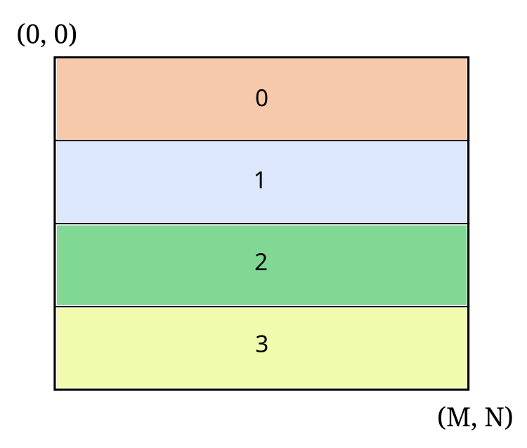
Here we see a MxN 2D array partitioned on the X axis, where each number (and color) denotes the slab of the global array owned by that process.

If \((M, N) = (40, 64)\), the shape of the slab on every process will be \((10, 64)\). For \((M, N) = (39, 64)\), the shape of the slab on the first three processes is \((10, 64)\) and the shape on the last process is \((9, 64)\).

Using the nvmath.distributed APIs, you can specify the above distribution like this:

from nvmath.distributed.distribution import Slab

distribution = Slab(partition_dim=0)
# or
distribution = Slab.X

Tip

We offer convenience aliases to use with 1D/2D/3D arrays: Slab.X, Slab.Y and Slab.Z (which partition on axis 0, 1 and 2, respectively).

Note

Slab is natively supported by cuFFTMp (distributed FFT API). A Slab (or compatible) distribution is recommended for best performance in cuFFTMp.

Box#

Given a global N-D array, a N-D box can be used to describe a subsection of the global array by indicating the lower and upper corner of the subsection. By associating boxes to processes we can describe a data distribution where every process owns a contiguous rectangular subsection of the global array.

For example, consider a 8x8 2D array distributed across 3 processes using the following boxes:

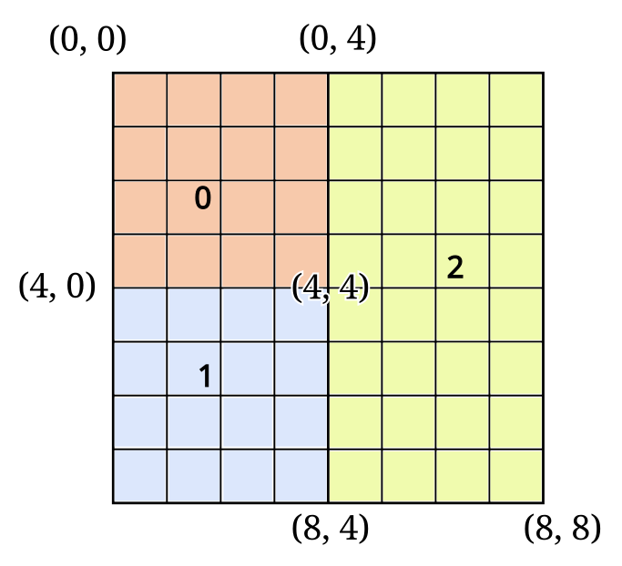
where each number (and color) denotes the subsection of the global N-D array owned by that process.

Using the nvmath.distributed APIs, you can specify the above distribution like this:

from nvmath.distributed.distribution import Box

if process_id == 0:
    distribution = Box((0, 0), (4, 4))
elif process_id == 1:
    distribution = Box((4, 0), (8, 4))
elif process_id == 2:
    distribution = Box((0, 4), (8, 8))

Note

Box is natively supported by cuFFTMp (distributed FFT and Reshape APIs). For further information, refer to the cuFFTMp documentation.

Block distributions#

In the block-cyclic distribution, a global N-D array is split into blocks of a specified shape and these blocks are distributed to a grid of processes in a cyclic pattern. As a result, each process owns a set of typically non-contiguous blocks of the global N-D array.

PBLAS uses the block-cyclic distribution to distribute dense matrices in a way that evenly balances the computational load across processes, while at the same time optimizing performance by being able to exploit memory locality (reference).

nvmath-python provides two distribution types based on block-cyclic, described below.

BlockCyclic#

BlockCyclic is specified with a process grid and a block size. The blocks assigned to a process are typically non-contiguous owing to the cyclic distribution pattern. Blocks can partition on any number of dimensions.

Consider the following example:

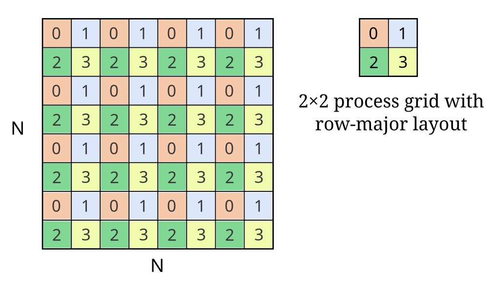
Here we see an NxN matrix distributed across 4 processes using a 2D block-cyclic scheme. Each number (and color) denotes the blocks of the global matrix belonging to that process. Each block has BxB elements and each process has 16 blocks.

Using the nvmath.distributed APIs, you can specify the above distribution like this:

from nvmath.distributed.distribution import ProcessGrid, BlockCyclic

process_grid = ProcessGrid(
    shape=(2, 2), layout=ProcessGrid.Layout.ROW_MAJOR
)
distribution = BlockCyclic(process_grid, (B, B))

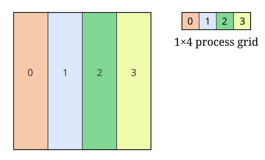
Note how the partition dimensions are determined by the process grid and block shape. Here is an example of 1D block-cyclic distribution:

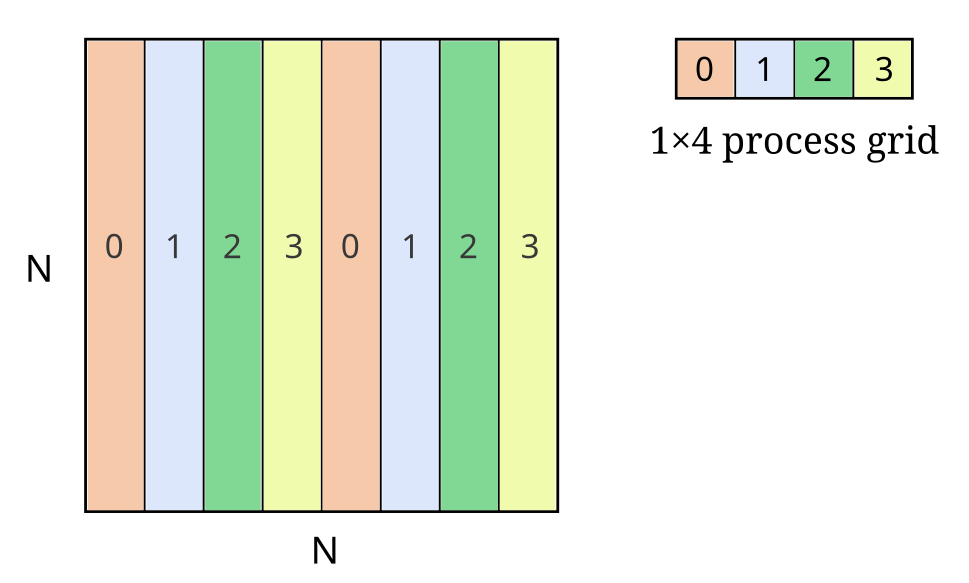
The above distribution can be specified like this:

from nvmath.distributed.distribution import ProcessGrid, BlockCyclic

# layout is irrelevant in this case and can be omitted
process_grid = ProcessGrid(shape=(1, 4))
distribution = BlockCyclic(process_grid, (N, B))

Note

Block distributions are natively supported by cuBLASMp (distributed matrix multiplication APIs).

BlockNonCyclic#

BlockNonCyclic is a special case of BlockCyclic, where the block size and process grid are such that it generates no cycles. For this distribution there is no need to specify block sizes, as nvmath-python can infer them automatically.

Tip

BlockNonCyclic is a convenience type and you can represent the same distribution with BlockCyclic and explicit block sizes.

Example 1D block non-cyclic:

The above distribution can be specified like this:

from nvmath.distributed.distribution import ProcessGrid, BlockNonCyclic

# layout is irrelevant in this case and can be omitted
process_grid = ProcessGrid(shape=(1, 4))
distribution = BlockNonCyclic(process_grid)

Note

Block distributions are natively supported by cuBLASMp (distributed matrix multiplication APIs).

Tip

Slab and BlockNonCyclic are equivalent for uniform partition sizes.

Utilities#

You can get the local shape of an operand according to a distribution by querying the distribution:

from nvmath.distributed.distribution import Slab

global_shape = (64, 48, 32)
# Get the local shape on this process according to Slab.Y
shape = Slab.Y.shape(process_id, global_shape)

If desired, you may do explicit conversion between distribution types. For example:

from nvmath.distributed.distribution import ProcessGrid, BlockNonCyclic, Slab

# layout is irrelevant in this case and can be omitted
process_grid = ProcessGrid(shape=(1, 4))
distribution = BlockNonCyclic(process_grid)
slab_distribution = distribution.to(Slab)
print(slab_distribution)  # prints "Slab(partition_dim=1, ndim=2)"

Distribution, memory layout and transpose#

Memory layout refers to the way that N-D arrays are stored in memory on each process. The two primary layouts are C-order (row-major) and Fortran-order (column-major). Memory layout is independent of the distribution of the global array, i.e. you can have any combination of distribution and local memory layout. In practice, however, math libraries have specific requirements on memory layout. For example, cuFFTMp requires C-order while cuBLASMp requires Fortran-order. As such, you may find that you have to convert the layout of your inputs. Two common ways to convert the layout are:

Copy the array to a buffer with the new layout (expensive, preserves the distribution).

For example:

# Get the local shape according to Slab.X
a_shape = Slab.X.shape(process_id, (m, n))
# Allocate operand on this process (NumPy uses C-order by default).
a = np.random.rand(*a_shape)
# Convert layout to F-order by copying to a new array (distribution is preserved)
a = np.asfortranarray(a)

Get a transposed view (efficient, modifies the distribution).

Transposing a global array transposes the distribution, and so always results in a different distribution. For example:

# Get the local shape according to Slab.X
a_shape = Slab.X.shape(process_id, (m, n))
# Allocate operand on this process (NumPy uses C-order by default).
a = np.random.rand(*a_shape)
# Transpose the global array (transposing on each process)
a = a.T  # the distribution of a is now Slab.Y

Note

Transposing changes the global shape of the operand and will accordingly impact the distributed operation. For example, if the global shape of the input matrix A of distributed matrix multiplication is \((k, m)\), you have to set the is_transpose qualifier to True for A. Similarly if B is transposed. See Distributed Linear Algebra for more information.

Hint

For matrices, transpose(Slab.X) == Slab.Y and transpose(Slab.Y) == Slab.X.

API Reference#

`Slab`(partition_dim[, ndim])	Slab distribution
`Box`(lower, upper)	Box distribution
`ProcessGrid`(*[, shape, layout, process_array])	N-dimensional grid of processes used by some distributions like the PBLAS block-cyclic distribution.
`BlockCyclic`(process_grid, block_sizes, *[, ...])	Block-cyclic distribution
`BlockNonCyclic`(process_grid, *[, first_process])	Block distribution without cycles