

3. Programming Model#
Tile IR extends CUDA’s low-level programming model with new abstractions that differ from what has previously existed in CUDA C++ or PTX.
This section introduces the programming model of Tile IR and familiarizes the reader with its core concepts and abstractions. We do this by working through a series of real programs, building up to a dynamic, high-performance implementation of GEMM that makes use of the major features of Tile IR.
Tile IR has an expressive tile-based programming model. We introduce users to the various ways to represent tensor computation by progressively adapting the example programs to take better advantage of Tile IR features which help simplify programs and enable the compiler to provide performance portability. We start by first introducing concepts that readers may be familiar with from prior art.
3.1. Tile Kernels#
Tile IR programs are referred to as tile kernels, which like CUDA C++ or PTX, are functions which run as N copies in parallel when invoked. The primary difference is the basic unit of execution: a tile-block, which expresses the computation performed by a single logical tile thread operating over a multi-dimensional tile of data.
During execution, each tile kernel is referred to as a tile kernel instance.
Below is a simple Tile IR kernel which prints “Hello World!”.
cuda_tile.module @hello_world_module {
    entry @hello_world_kernel() {
        print_tko "Hello World!\n" -> token
    }
}
For those familiar with CUDA threads, it is important to note that Tile IR’s threads are different. Before we go any further into formalisms, it is essential we highlight those differences.
Tile kernels are the entry point of the program, executing as parallel instances of tile blocks.
3.1.1. What’s different about tile programming?#
Tile IR is an extension to the CUDA programming model that enables first class support for tile programming. Tiled kernels express programs as a grid of logical tile threads that operate over tiles. The mapping of both the grid and individual tile threads to the underlying hardware’s threads is abstracted away from the programming model and is handled by the compiler.
The SIMT programming model of NVIDIA’s streaming multiprocessor (SM) is one in which threads operate over (relatively) small pieces of data and the user is responsible for dividing and scheduling the threads into the appropriate blocks to compute over the input data in an efficient manner. This model gives flexibility to programmers on how to map threads to data, or vice-versa. SIMT is the programming model exposed by CUDA and PTX and has served NVIDIA GPUs well since its introduction in 2006.
The rise in importance of deep learning has both introduced a greater regularity to user workloads and an ever increasing need to deliver performance for these workloads. As discussed in the Introduction, this has led to new specialized hardware in the form of tensor cores.
Tensor cores introduce a new dimension to the SIMT programming model. Now, SM threads must cooperate with the tensor cores in order to reach peak performance. With each new generation of hardware the interplay between these two pieces of silicon has unlocked amazing new performance but with increasing programming complexity.
Tile IR has been built to aid in the implementation of high-performance algorithms that take full advantage of the underlying hardware’s capabilities while mitigating the increase in programming complexity.
By abstracting thread-to-data mapping, Tile IR simplifies the use of specialized hardware like Tensor Cores compared to traditional SIMT models.
3.1.2. Kernel I/O#
To illustrate the design of Tile IR we will move from our simple hello world kernel
to one which implements 1-d tensor (i.e., vector) addition with a fixed block size
128. All examples presented in this section can be found in the
Programming Model Example Programs.
Tile kernels accept inputs and outputs as parameters; this is the only mechanism for consuming and producing data, so we start by defining the kernel parameters.
entry @vector_block_add_128x1_kernel(
    %a_ptr_base_scalar : !cuda_tile.tile<ptr<f32>>,
    %b_ptr_base_scalar : !cuda_tile.tile<ptr<f32>>,
    %c_ptr_base_scalar : !cuda_tile.tile<ptr<f32>>)
The above code fragment defines a kernel named vector_block_add_128x1_kernel which
takes three arguments, representing the two input buffers a and b, and the
output buffer c. Each argument is a rank-0 tile whose element type is a pointer.
Tile IR has three principal kinds of SSA values: tiles, views, and tokens (see Type System). A tile is an n-dimensional rectangular array of element values, described by its rank (number of dimensions), shape (extent along each dimension), and element type. Tiles may have rank 0 or higher; a rank-0 tile represents a scalar. A tile’s rank, dimensions, and element type are statically known. A pointer is an element type carried by a tile, not a separate kind of SSA value.
Views are structured descriptions of memory, rather than arrays of values themselves. A tensor view associates a base pointer with the shape and strides of an allocation, and a subview describes how operations access statically shaped tiles from that allocation. Tokens carry ordering dependencies between memory operations. Tile kernels do not have return values and therefore omit a return type annotation (tile functions may have return types and are discussed later).
An astute reader might now be wondering why we gave the inputs and outputs scalar pointer types instead of tensor-view types with statically known rank, shape, and stride. A common pattern in the Tile IR programming model is for kernels to take unstructured base pointers as parameters which can then be used to construct the required view or tile of pointers. This flexibility gives rise to multiple ways to use pointers depending on the desired program behavior, but we will first focus on the most flexible representation by converting our base pointer into a tile of arbitrary pointers. A tile of arbitrary pointers allows scatter/gather-style loads from a set of addresses at once.
We must take a few steps to convert a base pointer %a_ptr_base_scalar into a tile of
pointers representing the 128x1 tile we want to compute on which contains addresses
from (base + 0, ..., base + 127)
We start by creating an offset tile which represents the inclusive (0, 127)
interval. We use cuda_tile.iota which constructs a range tile that counts from
0 to n - 1 forming an n-element vector.
%offset = iota : tile<128xi32>
We then reshape from a scalar ptr<f32> to a 1-d tile 1xptr<f32> so we have the
correct rank.
%a_ptr_base_tensor = reshape %a_ptr_base_scalar :
    tile<ptr<f32>> -> tile<1xptr<f32>>
We then broadcast the pointer so we have a 1-d tile of (base, ..., base) containing
128 elements.
%a_ptr = broadcast %a_ptr_base_tensor : tile<1xptr<f32>> -> tile<128xptr<f32>>
Add the offset tile to the tile of pointers to obtain a tile<128xptr<f32>> that
contains pointers of (base + 0, ..., base + 127) as its values. Now we have a tile
of pointers which represents the tile that we would like to compute on. We perform the
same set of steps for a, b, and c.
%a_tensor = offset %a_ptr, %offset :
    tile<128xptr<f32>>, tile<128xi32> -> tile<128xptr<f32>>
Finally, we load both operands, perform the addition, and store to the output.
%a_val, %token_a = load_ptr_tko weak %a_tensor : tile<128xptr<f32>> -> tile<128xf32>, token
%b_val, %token_b = load_ptr_tko weak %b_tensor : tile<128xptr<f32>> -> tile<128xf32>, token
%c_val = addf %a_val, %b_val rounding<nearest_even> : tile<128xf32>
store_ptr_tko weak %c_tensor, %c_val : tile<128xptr<f32>>, tile<128xf32> -> token
We now have a complete kernel for a single tile-block that performs addition over 128 element vectors. As you can see this code is written from a single thread of control, but its level of parallelism will be determined by the compiler.
Kernels communicate with global memory via pointer arguments, which can be transformed into pointer tiles or tensor views for flexible data access.
3.2. Tile Grid#
So far we have only examined kernels which are written for a single tile block. Tile IR allows tile blocks to be grouped into a tile grid, similar to CUDA C++, enabling users to launch sets of tile blocks that execute in parallel. Tile kernels, as with PTX, are implicitly parameterized over the tile block coordinates (which can be queried via cuda_tile.get_tile_block_id) and can be 1-d, 2-d, or 3-d.
When a tile kernel is launched the user specifies the grid size, which determines the
number of tile blocks launched. The number of tile blocks launched is equal to the size
of the grid. For example if we launch our previous example with a (1, 1, 2) grid, we
will run an identical computation twice.
We can now look at an improved hello world program which shows off querying the grid size and coordinates.
cuda_tile.module @hello_world_module {
    // TileIR kernel function
    entry @hello_world_kernel() {
        // Step 1. Get the tile block ID
        %block_x_index, %block_y_index, %block_z_index = cuda_tile.get_tile_block_id : tile<i32>

        // Step 2. Get the tile block dimensions
        %block_dim_x, %block_dim_y, %block_dim_z = cuda_tile.get_num_tile_blocks : tile<i32>

        // Step 3. Print the tile block ID and dimensions. Each tile executes the
        // following print statement and prints a single line.
        cuda_tile.print_tko "Hello, I am tile <%i, %i, %i> in a kernel with <%i, %i, %i> tiles.\n",
            %block_x_index, %block_y_index, %block_z_index, %block_dim_x, %block_dim_y, %block_dim_z
            : tile<i32>, tile<i32>, tile<i32>,
              tile<i32>, tile<i32>, tile<i32> -> token
        }
}
Each tile kernel can be launched with a 1-d, 2-d, or 3-d grid. Each tile block can query its position in the grid using cuda_tile.get_tile_block_id and query the first, second, or third dimension index by varying the argument. Tile kernels can also observe the grid dimensions in a similar way using cuda_tile.get_num_tile_blocks.
If we use a grid that is (1, 1, 2) we will see two prints:
1      "Hello, I am tile <0, 0, 0> in a kernel with <1, 1, 2> tiles."
2      "Hello, I am tile <0, 0, 1> in a kernel with <1, 1, 2> tiles."
The tile grid organizes parallel execution of tile blocks, allowing kernels to scale across the problem size by querying their coordinates within the grid.
3.2.1. Implementing GEMM#
Now that we understand the basics concepts of the Tile IR programming model, we will introduce how to compute a 2-d GEMM for a single block, and then generalize it step by step to a full GEMM by utilizing the tile grid and introducing control flow and manual tiling.
This progression demonstrates how to compose basic tile operations into a complex, high-performance parallel algorithm.
3.2.2. GEMM with a Single Block#
Let’s first start by naturally moving from a single static block vector addition to a single static square block matrix multiplication.
This example proceeds much as before:
    entry @gemm_block_64x64_kernel(
        %a_ptr_base_scalar: !cuda_tile.tile<!cuda_tile.ptr<f32>>,
        %b_ptr_base_scalar: !cuda_tile.tile<!cuda_tile.ptr<f32>>,
        %c_ptr_base_scalar: !cuda_tile.tile<!cuda_tile.ptr<f32>>
    ) {
We start with a set of scalar pointers. To simplify this example, we assume that each
pointer refers to an allocation of at least 64 * 64 = 4096 contiguous elements.
Then much like before we declare a square offset tile.
    %offset_flat = iota : tile<4096xi32>
    %offset = reshape %offset_flat :
        tile<4096xi32> -> tile<64x64xi32>
We declare pointers to the underlying tiles the same way as before for A, B, C.
    %a_ptr_base_tensor = reshape %a_ptr_base_scalar :
        tile<ptr<f32>> -> tile<1x1xptr<f32>>
    %a_ptr = broadcast %a_ptr_base_tensor : tile<1x1xptr<f32>> -> tile<64x64xptr<f32>>
    %a_tensor = offset %a_ptr, %offset :
        tile<64x64xptr<f32>>, tile<64x64xi32> -> tile<64x64xptr<f32>>

    // Now we do the same for B.
    %b_ptr_base_tensor = reshape %b_ptr_base_scalar :
        tile<ptr<f32>> -> tile<1x1xptr<f32>>
    %b_ptr = broadcast %b_ptr_base_tensor : tile<1x1xptr<f32>> -> tile<64x64xptr<f32>>
    %b_tensor = offset %b_ptr, %offset :
        tile<64x64xptr<f32>>, tile<64x64xi32> -> tile<64x64xptr<f32>>

    // And the same for C.
    %c_ptr_base_tensor = reshape %c_ptr_base_scalar :
        tile<ptr<f32>> -> tile<1x1xptr<f32>>
    %c_ptr = broadcast %c_ptr_base_tensor : tile<1x1xptr<f32>> -> tile<64x64xptr<f32>>
    %c_tensor = offset %c_ptr, %offset :
         tile<64x64xptr<f32>>, tile<64x64xi32> -> tile<64x64xptr<f32>>
The only difference here is that we are building square tiles in 2D instead of 1D.
We then load the input arguments, compute the MMA operation (see cuda_tile.mmaf for floating-point and cuda_tile.mmai for integers) to compute the output tile, and then store it.
    // Load a single 64x64 matrix from the tile.
    %A_block, %token_a = load_ptr_tko weak %a_tensor :
        tile<64x64xptr<f32>> -> tile<64x64xf32>, token
    // Load a single 64x64 matrix from the tile.
    %B_block, %token_b = load_ptr_tko weak %b_tensor :
        tile<64x64xptr<f32>> -> tile<64x64xf32>, token
    %init_accum = cuda_tile.constant <f32: 0.000000e+00> : !cuda_tile.tile<64x64xf32>
    // Multiply A and B and accumulate from zero.
    %C_block = mmaf %A_block, %B_block, %init_accum: tile<64x64xf32>, tile<64x64xf32>, tile<64x64xf32>
    store_ptr_tko weak %c_tensor, %C_block :
        tile<64x64xptr<f32>>, tile<64x64xf32> -> token
If you are experienced in implementing matrix multiplication, you can see that this
works well for a single 64x64 square multiplication, but what happens if we want to
run the tile kernel over a large input problem size in parallel?
Basic matrix multiplication is achieved by constructing 2D tiles from pointers and performing matrix-multiply-accumulate (MMA) operations within a single block.
3.2.3. GEMM Block by Block#
We can generalize the single-block example to row-major 4096x4096 matrices. A
64x64 grid of tile blocks computes 64x64 output tiles; block_x selects the
output’s M tile and block_y selects its N tile. The kernel still receives scalar
base pointers.
entry @gemm_square_4096_tile_64x64_kernel(
    %a_ptr_base_scalar: tile<ptr<f32>>,
    %b_ptr_base_scalar: tile<ptr<f32>>,
    %c_ptr_base_scalar: tile<ptr<f32>>
) {
    // block_x selects the M tile and block_y selects the N tile.
    %block_x_index, %block_y_index, %block_z_index = get_tile_block_id : tile<i32>
The full row-major matrices have strides (4096, 1). The kernel also creates a range
[0, 64) used for coordinates within each tile, loop bounds for the 64 K tiles, and a
zero accumulator.
%tile_size = constant <i32: 64> : tile<i32>
%matrix_stride = constant <i32: 4096> : tile<64x64xi32>
%range_start = constant <i32: 0> : tile<i32>
%range_end = constant <i32: 64> : tile<i32>
%range_step = constant <i32: 1> : tile<i32>
%init_accum = constant <f32: 0.000000e+00> : tile<64x64xf32>
%tile_size_range = iota : tile<64xi32>
For A, the row coordinates are block_x * 64 + arange(0, 64). Broadcasting those
coordinates down the columns and multiplying by the full row stride gives the row
contribution. The K coordinate is contiguous, so adding a broadcast of arange(0, 64)
gives A[m, k] = m * 4096 + k.
// Compute A's row coordinates:
//   m = block_x * 64 + arange(0, 64)
%a_tile_base = muli %block_x_index, %tile_size : tile<i32>
%a_tile_base_reshape = reshape %a_tile_base :
    tile<i32> -> tile<1xi32>
%a_tile_base_tensor = broadcast %a_tile_base_reshape :
    tile<1xi32> -> tile<64xi32>
%m_offsets_vec = addi %a_tile_base_tensor, %tile_size_range :
    tile<64xi32>

// A is row-major, so A[m, k] has offset m * 4096 + k.
%m_offsets_matrix = reshape %m_offsets_vec :
    tile<64xi32> -> tile<64x1xi32>
%m_offsets_broadcast = broadcast %m_offsets_matrix :
    tile<64x1xi32> -> tile<64x64xi32>
%m_offsets = muli %m_offsets_broadcast, %matrix_stride :
    tile<64x64xi32>

%ak_offsets_matrix = reshape %tile_size_range :
     tile<64xi32> -> tile<1x64xi32>
%ak_offsets = broadcast %ak_offsets_matrix :
    tile<1x64xi32> -> tile<64x64xi32>

%a_tile_offsets = addi %m_offsets, %ak_offsets : tile<64x64xi32>
For B, the N coordinates are block_y * 64 + arange(0, 64). K is B’s row dimension,
so its contribution is multiplied by 4096; N remains contiguous. The sum gives B[k, n]
= k * 4096 + n.
// Compute B's column coordinates:
//   n = block_y * 64 + arange(0, 64)
%b_tile_base = muli %block_y_index, %tile_size : tile<i32>
%b_tile_base_reshape = reshape %b_tile_base :
    tile<i32> -> tile<1xi32>
%b_tile_base_tensor = broadcast %b_tile_base_reshape :
    tile<1xi32> -> tile<64xi32>
%n_offsets_vec = addi %b_tile_base_tensor, %tile_size_range :
    tile<64xi32>

// B is row-major, so B[k, n] has offset k * 4096 + n.
%bk_offsets_matrix = reshape %tile_size_range :
    tile<64xi32> -> tile<64x1xi32>
%bk_offsets_broadcast = broadcast %bk_offsets_matrix :
    tile<64x1xi32> -> tile<64x64xi32>
%bk_offsets = muli %bk_offsets_broadcast, %matrix_stride :
    tile<64x64xi32>

%n_offsets_matrix = reshape %n_offsets_vec :
    tile<64xi32> -> tile<1x64xi32>
%n_offsets = broadcast %n_offsets_matrix :
    tile<1x64xi32> -> tile<64x64xi32>

%b_tile_offsets = addi %bk_offsets, %n_offsets : tile<64x64xi32>
The two offset matrices are applied to broadcast base pointers to create the initial pointer tiles.
// Form the initial pointer tiles for A and B.
%a_ptr_base_tensor = reshape %a_ptr_base_scalar :
    tile<ptr<f32>> -> tile<1x1xptr<f32>>
%a_ptr = broadcast %a_ptr_base_tensor :
    tile<1x1xptr<f32>> -> tile<64x64xptr<f32>>
%a_tile_ptr = offset %a_ptr, %a_tile_offsets :
    tile<64x64xptr<f32>>, tile<64x64xi32> -> tile<64x64xptr<f32>>

%b_ptr_base_tensor = reshape %b_ptr_base_scalar :
    tile<ptr<f32>> -> tile<1x1xptr<f32>>
%b_ptr = broadcast %b_ptr_base_tensor :
    tile<1x1xptr<f32>> -> tile<64x64xptr<f32>>
%b_tile_ptr = offset %b_ptr, %b_tile_offsets :
    tile<64x64xptr<f32>>, tile<64x64xi32> -> tile<64x64xptr<f32>>
3.2.4. Looping Over Tiles#
The reduction contains 64 K tiles. On each iteration the kernel loads A and B,
accumulates an MMA, then advances A by 64 elements along each row and B by 64 * 4096
elements (64 complete rows). Crucially, the loads consume the loop-carried pointer
values, and the loop step is one.
// There are 4096 / 64 = 64 tiles along K.  Advancing A moves 64
// elements along a row; advancing B moves 64 complete rows.
%a_k_advance = constant <i32: 64> : tile<64x64xi32>
%b_k_advance = constant <i32: 262144> : tile<64x64xi32>
%C_tile, %a_ptr_final, %b_ptr_final = for %k in
    (%range_start to %range_end, step %range_step) : tile<i32>
    iter_values(
        %acc_prev = %init_accum,
        %a_tile_ptr_prev = %a_tile_ptr,
        %b_tile_ptr_prev = %b_tile_ptr
    ) -> (tile<64x64xf32>, tile<64x64xptr<f32>>, tile<64x64xptr<f32>>)
{
    %A_tile, %token_a = load_ptr_tko weak %a_tile_ptr_prev :
        tile<64x64xptr<f32>> -> tile<64x64xf32>, token
    %B_tile, %token_b = load_ptr_tko weak %b_tile_ptr_prev :
        tile<64x64xptr<f32>> -> tile<64x64xf32>, token

    %C_tile_acc = mmaf %A_tile, %B_tile, %acc_prev :
        tile<64x64xf32>, tile<64x64xf32>, tile<64x64xf32>
    %a_tile_ptr_next = offset %a_tile_ptr_prev, %a_k_advance :
        tile<64x64xptr<f32>>, tile<64x64xi32> -> tile<64x64xptr<f32>>
    %b_tile_ptr_next = offset %b_tile_ptr_prev, %b_k_advance :
        tile<64x64xptr<f32>>, tile<64x64xi32> -> tile<64x64xptr<f32>>
    continue %C_tile_acc, %a_tile_ptr_next, %b_tile_ptr_next :
        tile<64x64xf32>, tile<64x64xptr<f32>>, tile<64x64xptr<f32>>
}
Finally, C uses the same output M and N coordinates. Its row contribution is multiplied by 4096, its column contribution is contiguous, and those contributions are added before storing the accumulated tile.
// C is row-major, so C[m, n] has offset m * 4096 + n.
%c_tile_x_start = muli %block_x_index, %tile_size : tile<i32>
%c_tile_x_start_reshape = reshape %c_tile_x_start :
    tile<i32> -> tile<1xi32>
%c_tile_x_start_tensor = broadcast %c_tile_x_start_reshape :
    tile<1xi32> -> tile<64xi32>
%c_tile_x_offsets_vec = addi %c_tile_x_start_tensor, %tile_size_range :
    tile<64xi32>

%c_tile_y_start = muli %block_y_index, %tile_size : tile<i32>
%c_tile_y_start_reshape = reshape %c_tile_y_start :
    tile<i32> -> tile<1xi32>
%c_tile_y_start_tensor = broadcast %c_tile_y_start_reshape :
    tile<1xi32> -> tile<64xi32>
%c_tile_y_offsets_vec = addi %c_tile_y_start_tensor, %tile_size_range :
    tile<64xi32>

%c_tile_x_offsets_matrix = reshape %c_tile_x_offsets_vec :
    tile<64xi32> -> tile<64x1xi32>
%c_tile_x_offsets_broadcast = broadcast %c_tile_x_offsets_matrix :
    tile<64x1xi32> -> tile<64x64xi32>
%c_tile_x_offsets = muli %c_tile_x_offsets_broadcast, %matrix_stride :
    tile<64x64xi32>

%c_tile_y_offsets_matrix = reshape %c_tile_y_offsets_vec :
    tile<64xi32> -> tile<1x64xi32>
%c_tile_y_offsets = broadcast %c_tile_y_offsets_matrix :
    tile<1x64xi32> -> tile<64x64xi32>
%c_tile_offsets = addi %c_tile_x_offsets, %c_tile_y_offsets :
    tile<64x64xi32>

%c_ptr_base_tensor = reshape %c_ptr_base_scalar :
    tile<ptr<f32>> -> tile<1x1xptr<f32>>
%c_ptr = broadcast %c_ptr_base_tensor :
    tile<1x1xptr<f32>> -> tile<64x64xptr<f32>>
%c_tile_ptr = offset %c_ptr, %c_tile_offsets :
    tile<64x64xptr<f32>>, tile<64x64xi32> -> tile<64x64xptr<f32>>

store_ptr_tko weak %c_tile_ptr, %C_tile :
    tile<64x64xptr<f32>>, tile<64x64xf32> -> token
This explicit-pointer example illustrates every address calculation. The view-based examples later in this chapter express the same mapping through shape, stride, and tile metadata.
3.3. Tensor Views#
The previous examples use arbitrary tiles of pointers. That representation is fully general, but constructing every address manually obscures regular memory structure from both the reader and the compiler. In the worst case, each element may become a disjoint memory operation with little opportunity for coalescing or locality-aware lowering.
A tensor view is Tile IR’s structured memory abstraction. It associates a scalar base pointer with tensor shape and stride metadata, simplifying the program while exposing the access pattern to the compiler.

The base pointer to A points to an allocation that lives in global memory.#
A tensor view is constructed from a raw pointer with cuda_tile.make_tensor_view. Its shape and strides may contain both static and runtime values. Subsequent subview operations describe how that logical tensor is divided into tiles used by load and store operations.
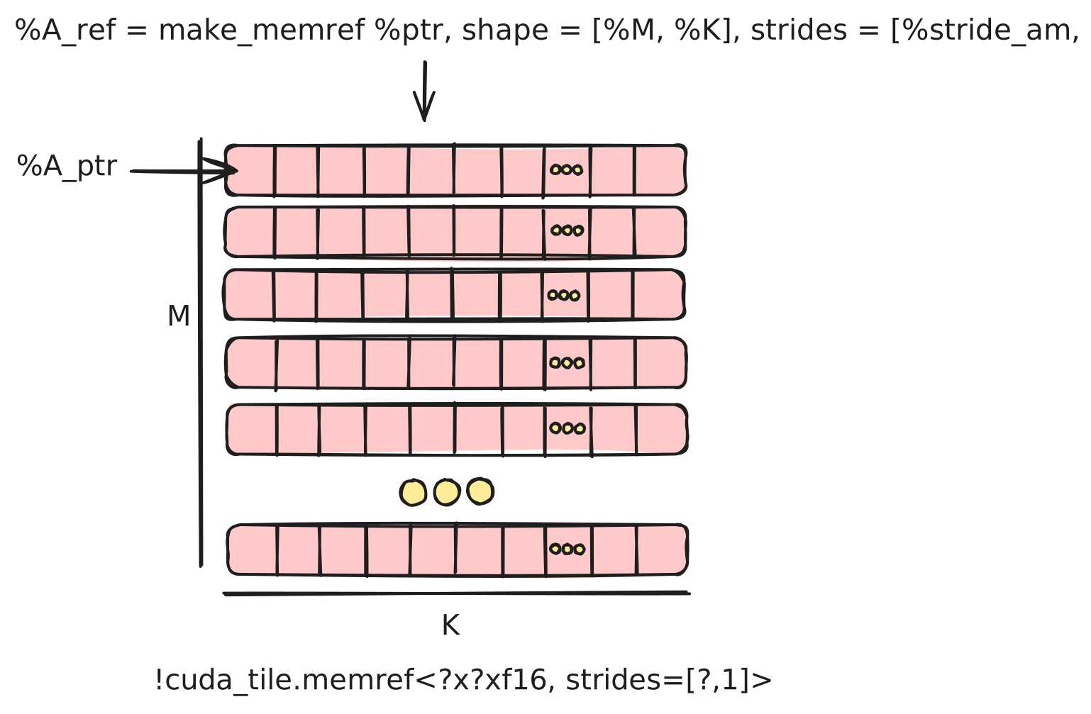
The base pointer to A points to an allocation that lives in global memory.#
Tensor views encapsulate shape and stride information, enabling the compiler to optimize memory access while simplifying the user’s code.
3.4. Tiling & Views#
Once you have constructed a tensor view, we can make use of cuda_tile.make_partition_view to perform tiling of the underlying tensor.
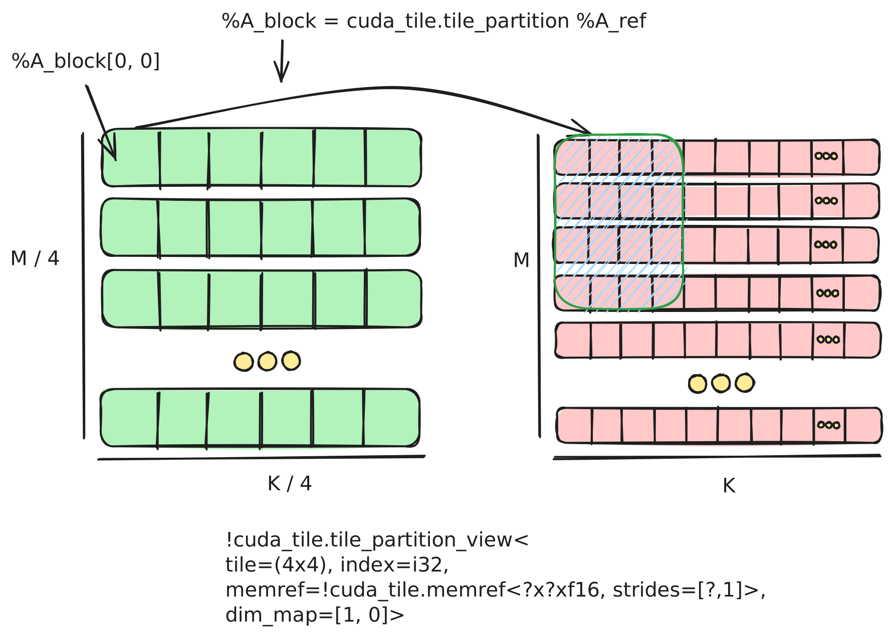
The base pointer to A points to an allocation that lives in global memory.#
In the last section we simplified the problem by choosing tile dimensions that made the problem perfectly square, in the same layout, using simple tiling and static input dimensions, etc. We will relax those constraints to show more complex tile mappings as we explore views and partitions.
3.4.1. Vector Addition with Views#
We can now implement a more complex vector operation with SAXPY, or “Single-Precision A·X Plus Y” (a common BLAS operation). We can use tensor views and cuda_tile.make_partition_view to implement this operation for arbitrary sized vectors.
The kernel first defines its arguments. We now take the inputs %X, %Y,
%alpha, as well as the dimensions of the full vectors, as arguments.
entry @saxpy(%X: tile<ptr<f32>>,
                    %Y: tile<ptr<f32>>,
                    %alpha: tile<f32>,
                    %M : tile<i32>,
                    %N : tile<i32>) {
For those familiar with other tile programming models, you might wonder why we need to take the input tensor sizes as arguments instead of using them to control the number of blocks and remain implicit in the program.
The tensor view model differs from some existing tile programming models, wherein each kernel is unaware of the overall dimensions of the problem size beyond the need to mask loads and stores. In contrast, tensor views require the overall tensor dimensions in order to enable efficient and correct lowering of tiling and its related operations automatically.
%x_tensor_view = make_tensor_view %X, shape = [%M, %N], strides = [%N, 1] : tile<i32> -> tensor_view<?x?xf32, strides=[?,1]>
%y_tensor_view = make_tensor_view %Y, shape = [%M, %N], strides = [%N, 1] : tile<i32> -> tensor_view<?x?xf32, strides=[?,1]>
The tensor-view constructor accepts runtime shapes and strides, resulting in a
dynamically shaped view. A ? marks each dynamic component, as in
!cuda_tile.tensor_view<?x?xf32, strides=[?, 1]>.
We use cuda_tile.make_partition_view to create views for %x and %y
which have an index-space shape of (ceildiv(M, 128) x ceildiv(N, 256)). Each tile
will have the size specified by the tile parameter of the partition type.
%x_view = make_partition_view %x_tensor_view : partition_view<tile=(128x256), tensor_view<?x?xf32, strides=[?,1]>>
%y_view = make_partition_view %y_tensor_view : partition_view<tile=(128x256), tensor_view<?x?xf32, strides=[?,1]>>
cuda_tile.load_view_tko allows us to load the tile specified by %view[%x,
%y] for both %X and %Y.
%x_tile, %token_x = load_view_tko weak %x_view[%tileIdX, %tileIdY] :
    partition_view<tile=(128x256), tensor_view<?x?xf32, strides=[?,1]>>, tile<i32> -> tile<128x256xf32>, token
%y_tile, %token_y = load_view_tko weak %y_view[%tileIdX, %tileIdY] :
    partition_view<tile=(128x256), tensor_view<?x?xf32, strides=[?,1]>>, tile<i32> -> tile<128x256xf32>, token
We can then simply compute using the tiles directly to obtain our result tile.
// Step 6. Compute SAXPY: y = alpha * X + y
%9 = mulf %alpha_tensor, %x_tile rounding<nearest_even> : tile<128x256xf32>
%result_tile = addf %9, %y_tile rounding<nearest_even> : tile<128x256xf32>
Finally we accumulate the result into %Y directly. Here we treat it as both an input
and output parameter in this kernel.
// Step 7. Store the result tile to Y
store_view_tko weak %result_tile, %y_view[%tileIdX, %tileIdY] :
    tile<128x256xf32>, partition_view<tile=(128x256), tensor_view<?x?xf32, strides=[?,1]>>, tile<i32> -> token
Combining tensor views with partitioning simplifies kernel implementation, allowing direct loading and operating on logical tiles without manual offset arithmetic.
3.4.2. Dynamic GEMM with Views#
We have now introduced the core concepts of Tile IR. We can put together many of
these ideas to support a dynamic GEMM kernel using tensor views. To start, we make two
changes to this GEMM: the inputs are actually transposed into column-major layout, and
the inputs are in fp16 while the output is in fp32.
We take the input and output buffers as pointers, along with all dimensions and strides.
    entry @gemm_kloop_kernel(
        %A_ptr: !cuda_tile.tile<!cuda_tile.ptr<f16>>,
        %B_ptr: !cuda_tile.tile<!cuda_tile.ptr<f16>>,
        %C_ptr: !cuda_tile.tile<!cuda_tile.ptr<f32>>,
        %M: !cuda_tile.tile<i32>, %N: !cuda_tile.tile<i32>, %K: !cuda_tile.tile<i32>,
        %stride_ak: !cuda_tile.tile<i32>, %stride_bn: !cuda_tile.tile<i32>, %stride_cm: !cuda_tile.tile<i32>
    ) {
The Tile IR compiler can optimize the memory loads and stores of cuda_tile.tensor_view if the alignment of the underlying pointers and strides are known. If these are statically known then we can infer the alignment directly but if they are dynamic, as they are in this case, we can use the cuda_tile.assume operation to inform the compiler that the pointer is properly aligned.
Here we use the div_by predicate to inform the compiler about the divisibility of
these values which can be used to infer alignment constraints directly.
%A_ptr_assume = assume #cuda_tile.div_by<16>, %A_ptr : tile<ptr<f16>>
%B_ptr_assume = assume #cuda_tile.div_by<16>, %B_ptr : tile<ptr<f16>>
%C_ptr_assume = assume #cuda_tile.div_by<16>, %C_ptr : tile<ptr<f32>>
%stride_ak_assume = assume #cuda_tile.div_by<8>, %stride_ak : tile<i32>
%stride_bn_assume = assume #cuda_tile.div_by<8>, %stride_bn : tile<i32>
%stride_cm_assume = assume #cuda_tile.div_by<8>, %stride_cm : tile<i32>
We create a tensor view for %A, %B, and %C.
// A reference to the A tensor pointed to by A_ptr, (K x M)
%A = make_tensor_view %A_ptr_assume, shape = [%K, %M], strides = [%stride_ak, 1] : tile<i32> -> tensor_view<?x?xf16, strides=[?,1]>
// A reference to the B tensor pointed to by B_ptr, (N x K)
%B = make_tensor_view %B_ptr_assume, shape = [%N, %K], strides = [%stride_bn, 1] : tile<i32> -> tensor_view<?x?xf16, strides=[?,1]>
// A reference to the C tensor pointed to by C_ptr, (M x N)
%C = make_tensor_view %C_ptr_assume, shape = [%M, %N], strides = [%stride_cm, 1] : tile<i32> -> tensor_view<?x?xf32, strides=[?,1]>
We create a cuda_tile.partition_view for each tensor view. First A:
%A_block = make_partition_view %A : partition_view<tile=(128x64), padding_value = zero, tensor_view<?x?xf16, strides=[?,1]>, dim_map=[1, 0]>
Then B:
%B_block = make_partition_view %B : partition_view<tile=(64x128), padding_value = zero, tensor_view<?x?xf16, strides=[?,1]>, dim_map=[1, 0]>
And last C:
%C_block = make_partition_view %C : partition_view<tile=(128x128), tensor_view<?x?xf32, strides=[?,1]>, dim_map=[0, 1]>
We then read the tile block grid coordinates using cuda_tile.get_tile_block_id.
%bidx, %bidy, %bidz = get_tile_block_id : tile<i32>
Because the K dimension is dynamic, the size of the reduction index space must be
computed at runtime. cuda_tile.get_index_space_shape returns this size and
therefore the number of iterations in the reduction loop.
%mk_len_i32:2 = get_index_space_shape %A_block : partition_view<tile=(128x64), padding_value = zero, tensor_view<?x?xf16, strides=[?,1]>, dim_map=[1, 0]> -> tile<i32>
Now we can use a cuda_tile.for loop to iterate over the tiles.
A for loop is one of the structured control-flow operations in Tile IR. It steps
a loop variable over a range (start, end, step), executing the body for each value
in the range. The iter_values are loop-carried variables initialized in the loop
header and updated each iteration by yielding them with the cuda_tile.continue
operation.
In order to implement the reduction we start from 0 to the size of the tiled K
dimension, stepping uniformly by 1 on each step and a single loop carried variable
representing the accumulator tile.
%result = for %k in (%i0 to %mk_len_i32#1, step %i1) : tile<i32>
    iter_values(%acc_prev = %cst) -> (tile<128x128xf32>)
{
We load tiles from A and B. Both input partition views use zero padding, so an
incomplete final tile along the dynamic K dimension contributes zero rather than
unspecified out-of-bounds values.
// Load a single 128x64 matrix from the tile.
%A_frag, %t1 = load_view_tko weak %A_block[%bidx, %k] : partition_view<tile=(128x64), padding_value = zero, tensor_view<?x?xf16, strides=[?,1]>, dim_map=[1, 0]>, tile<i32> -> tile<128x64xf16>, token
// Load a single 64x128 matrix from the tile.
%B_frag, %t2 = load_view_tko weak %B_block [%k, %bidy] : partition_view<tile=(64x128), padding_value = zero, tensor_view<?x?xf16, strides=[?,1]>, dim_map=[1, 0]>, tile<i32> -> tile<64x128xf16>, token
We compute the MMA, and then continue to the next loop iteration with the value.
    %acc = mmaf %A_frag, %B_frag, %acc_prev: tile<128x64xf16>, tile<64x128xf16>, tile<128x128xf32>
    continue %acc : tile<128x128xf32>
Finally, like our previous implementation, outside the loop we store the tile back to
%C through its view, avoiding the need to compute the offsets again.
%t3 = store_view_tko weak %result, %C_block[%bidx, %bidy] : tile<128x128xf32>, partition_view<tile=(128x128), tensor_view<?x?xf32, strides=[?,1]>, dim_map=[0, 1]>, tile<i32> -> token
Tensor views support dynamic shapes and strides, enabling robust, flexible kernels that handle varying input sizes while maintaining high performance.
3.5. Cross TileBlock Communication#
  cuda_tile.module @hello_cross_block {
    global @_global_printf_mutex <i32: 1> : tile<1xi32>

    entry @hello_cross_block_kernel() {
      %idx, %idy, %idz = get_tile_block_id : tile<i32>
      %tilex, %tiley, %tilez = get_num_tile_blocks : tile<i32>
      %2 = get_global @_global_printf_mutex : tile<ptr<i32>>
      %3 = cuda_tile.constant <i32: 0> : tile<i32>
      %4 = cuda_tile.constant <i32: 1> : tile<i32>
      loop {
        %t1 = make_token : token
        %6, %t2 = atomic_cas_tko relaxed device %2, %4, %3 token=%t1: tile<!cuda_tile.ptr<i32>>, tile<i32> -> tile<i32>, !cuda_tile.token
        %7 = trunci %6 : tile<i32> -> tile<i1>
        if %7 {
          break
        }
      }
      %t3 = print_tko "current tile: %i / %i\0A", %idx, %tilex : tile<i32>, tile<i32> -> token
      %5, %t4 = atomic_rmw_tko relaxed device %2, xchg, %4 token=%t3 : tile<ptr<i32>>, tile<i32> -> tile<i32>, !cuda_tile.token
      return
    }
  }