Using FP8 and FP4 with Transformer Engine
H100 GPU introduced support for a new datatype, FP8 (8-bit floating point), enabling higher throughput of matrix multiplies and convolutions. Blackwell added support for NVFP4 and MXFP8 datatypes. In this example we will introduce these low precision datatypes and show how to use them with Transformer Engine.
Introduction to FP8
Structure
The FP8 datatype supported by H100 is actually 2 distinct datatypes, useful in different parts of the training of neural networks:
E4M3 - it consists of 1 sign bit, 4 exponent bits and 3 bits of mantissa. It can store values up to +/-448 and
nan.E5M2 - it consists of 1 sign bit, 5 exponent bits and 2 bits of mantissa. It can store values up to +/-57344, +/-
infandnan. The tradeoff of the increased dynamic range is lower precision of the stored values.
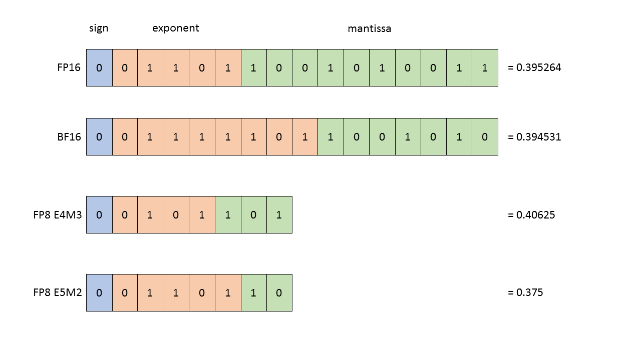
Figure 1: Structure of the floating point datatypes. All of the values shown (in FP16, BF16, FP8 E4M3 and FP8 E5M2) are the closest representations of value 0.3952.
During training neural networks both of these types may be utilized. Typically forward activations and weights require more precision, so E4M3 datatype is best used during forward pass. In the backward pass, however, gradients flowing through the network typically are less susceptible to the loss of precision, but require higher dynamic range. Therefore they are best stored using E5M2 data format. H100 TensorCores provide support for any combination of these types as the inputs, enabling us to store each tensor using its preferred precision.
Mixed precision training - a quick introduction
In order to understand how FP8 can be used for training Deep Learning models, it is useful to first remind ourselves how mixed precision works with other datatypes, especially FP16.
Mixed precision recipe for FP16 training has 2 components: choosing which operations should be performed in FP16 and dynamic loss scaling.
Choosing the operations to be performed in FP16 precision requires analysis of the numerical behavior of the outputs with respect to inputs of the operation as well as the expected performance benefit. This enables marking operations like matrix multiplies, convolutions and normalization layers as safe, while leaving
normorexpoperations as requiring high precision.Dynamic loss scaling enables avoiding both over- and underflows of the gradients during training. Those may happen since, while the dynamic range of FP16 is enough to store the distribution of the gradient values, this distribution may be centered around values too high or too low for FP16 to handle. Scaling the loss shifts those distributions (without affecting numerics by using only powers of 2) into the range representable in FP16.
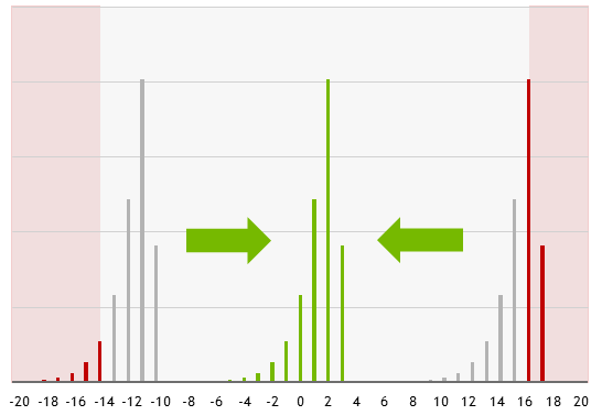
Figure 2: Scaling the loss enables shifting the gradient distribution into the representable range of FP16 datatype.
Mixed precision training with FP8
While the dynamic range provided by the FP8 types is sufficient to store any particular activation or gradient, it is not sufficient for all of them at the same time. This makes the single loss scaling factor strategy, which worked for FP16, infeasible for FP8 training and instead requires using distinct scaling factors for each FP8 tensor.
There are multiple strategies for choosing a scaling factor that is appropriate for a given FP8 tensor:
just-in-time scaling. This strategy chooses the scaling factor based on the maximum of absolute values (amax) of the tensor being produced. In practice it is infeasible, as it requires multiple passes through data - the operator produces and writes out the output in higher precision, then the maximum absolute value of the output is found and applied to all values in order to obtain the final FP8 output. This results in a lot of overhead, severely diminishing gains from using FP8.
delayed scaling. This strategy chooses the scaling factor based on the maximums of absolute values seen in some number of previous iterations. This enables full performance of FP8 computation, but requires storing the history of maximums as additional parameters of the FP8 operators.
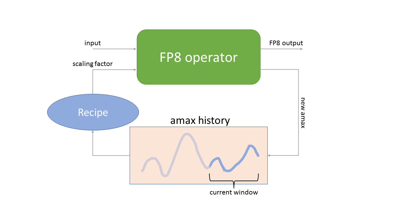
Figure 3: Delayed scaling strategy. The FP8 operator uses scaling factor obtained using the history of amaxes (maximums of absolute values) seen in some number of previous iterations and produces both the FP8 output and the current amax, which gets stored in the history.
As one can see in Figure 3, delayed scaling strategy requires both storing the history of amaxes, but also choosing a recipe for converting that history into the scaling factor used in the next iteration.
MXFP8 and block scaling
NVIDIA Blackwell architecture introduced support for a new variant of the FP8 format: MXFP8.
MXFP8 vs FP8
The main difference between “regular” FP8 and MXFP8 lies in the granularity of the scaling. In FP8, each tensor has a single FP32 scaling factor, so all values in the tensor need to “fit” within the dynamic range of the FP8 datatype. This requires using the less precise E5M2 format to represent some tensors in the network (like gradients).
MXFP8 addresses this by assigning a different scaling factor to each block of 32 consecutive values. This allows all values to be represented with the E4M3 datatype.
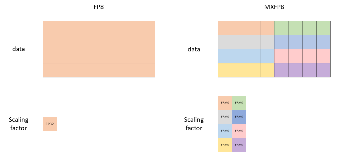
Figure 4: MXFP8 uses multiple scaling factors for a single tensor. The picture shows only 4 values per block for simplicity, but real MXFP8 has 32 values per block.
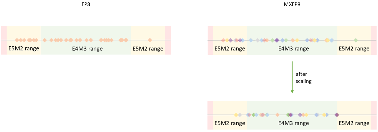
Figure 5: Due to multiple scaling factors, tensor’s dynamic range requirements are reduced and so E4M3 format can be used as far fewer elements get saturated to 0.
The second difference is the datatype used to store the scaling factors. FP8 uses FP32 (E8M23) while MXFP8 uses an 8-bit representation of a power of 2 (E8M0).
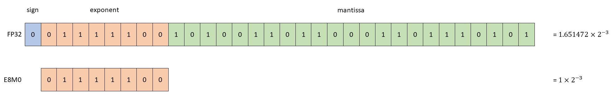
Figure 6: Structure of the E8M0 datatype used for storing scaling factors in MXFP8.
Handling transposes
The forward and backward passes of linear layers involve multiple matrix multiplications with different reduction dimensions. Blackwell Tensor Cores require MXFP8 data to be “consecutive” over the reduction dimension, so MXFP8 training uses non-transposed and transposed MXFP8 tensors at different points. However, while transposing FP8 data is numerically trivial, transposing MXFP8 data requires requantization.
To avoid loss of precision connected with this double quantization, Transformer Engine creates both regular and transposed copies of the tensor from the original high precision input.
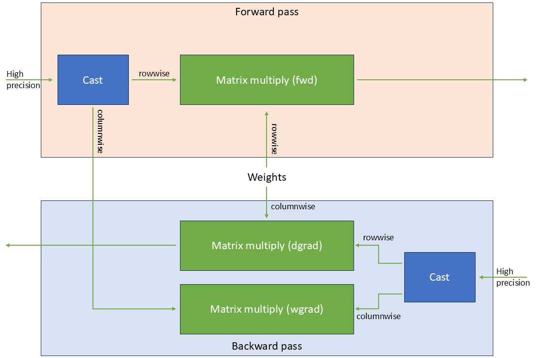
Figure 7: Linear layer in MXFP8. Calculating both forward and backward pass requires tensors quantized in both directions.
Beyond FP8 - training with NVFP4
In addition to MXFP8, NVIDIA Blackwell introduced support for an even smaller, 4-bit format called NVFP4. The values are represented there in E2M1 format, able to represent values of magnitude up to +/-6.
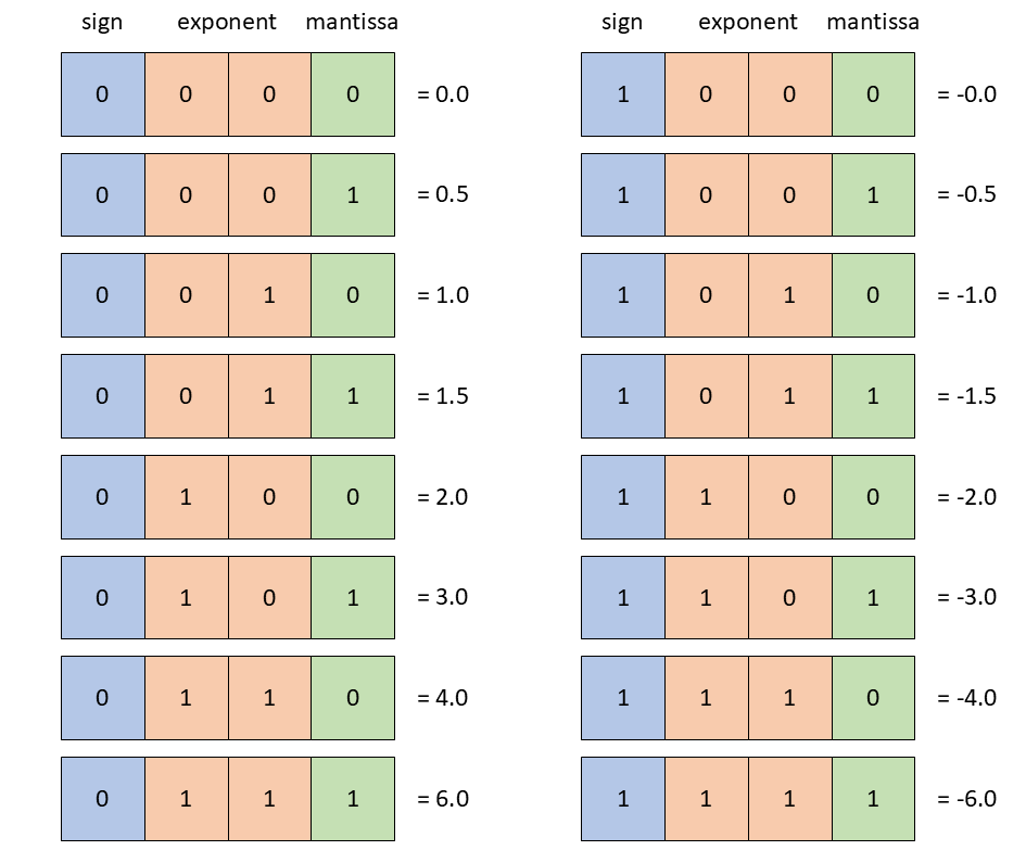
Figure 8: FP4 E2M1 format can represent values between +/-6.
NVFP4 Format
NVFP4 format is similar to MXFP8 - it also uses granular scaling to preserve the dynamic range. The differences are:
Granularity of the scaling factors: in NVFP4 format a single scaling factor is used per block of 16 elements, whereas MXFP8 uses 1 scaling factor per block of 32 elements
Datatype of the scaling factors: NVFP4 uses FP8 E4M3 as the scaling factor per block, whereas MXFP8 uses E8M0 as the scaling factor datatype. Choice of E4M3 for the scaling factor enables preservation of more information about mantissa, but does not enable the full dynamic range of FP32. Therefore, NVFP4 uses an additional single per-tensor FP32 scaling factor to avoid overflows.
In the NVFP4 training recipe for weight tensors we use a different variant of the NVFP4 quantization, where a single scaling factor is shared by a 2D block of 16x16 elements. This is similar to the weight quantization scheme employed in DeepSeek-v3 training, but with a much finer granularity.
NVFP4 training recipe
The NVFP4 training recipe implemented in Transformer Engine is described in Pretraining Large Language Models with NVFP4 paper. The main elements of the recipe are:
Stochastic Rounding. When quantizing gradients to NVFP4, we use stochastic rounding to avoid the bias introduced by quantization. With stochastic rounding values are rounded probabilistically to one of their two nearest representable numbers, with probabilities inversely proportional to their distances.
2D Scaling. The non-square size of the quantization blocks, while increasing granularity, has a property that the quantized tensor and its transpose no longer hold the same values. This is important since the transposed tensors are used when calculating gradients of the linear layers. While most tensors are not sensitive to this issue during training, it does affect the training accuracy when applied to the weight tensors. Therefore, the weights of the linear layers are quantized using a 2D scheme, where a single scaling factor is shared by a 2D block of 16x16 elements.
Random Hadamard Transforms. While microscaling reduces the dynamic range needed to represent tensor values, outliers can still have a disproportionate impact on FP4 formats, degrading model accuracy. Random Hadamard transforms address this by reshaping the tensor distribution to be more Gaussian-like, which smooths outliers and makes tensors easier to represent accurately in NVFP4. In Transformer Engine, we use a 16x16 Hadamard matrix for activations and gradients when performing weight gradient computation.
Last few layers in higher precision. The last few layers of the LLM are more sensitive to the quantization and so we recommend running them in higher precision (for example MXFP8). This is not done automatically in Transformer Engine, since TE does not have the full information about the structure of the network being trained. This can be easily achieved though by modifying the model training code to run the last few layers under a different
autocast(or nesting 2 autocasts in order to override the recipe for a part of the network).
The full linear layer utilizing NVFP4 is presented in Figure 9.
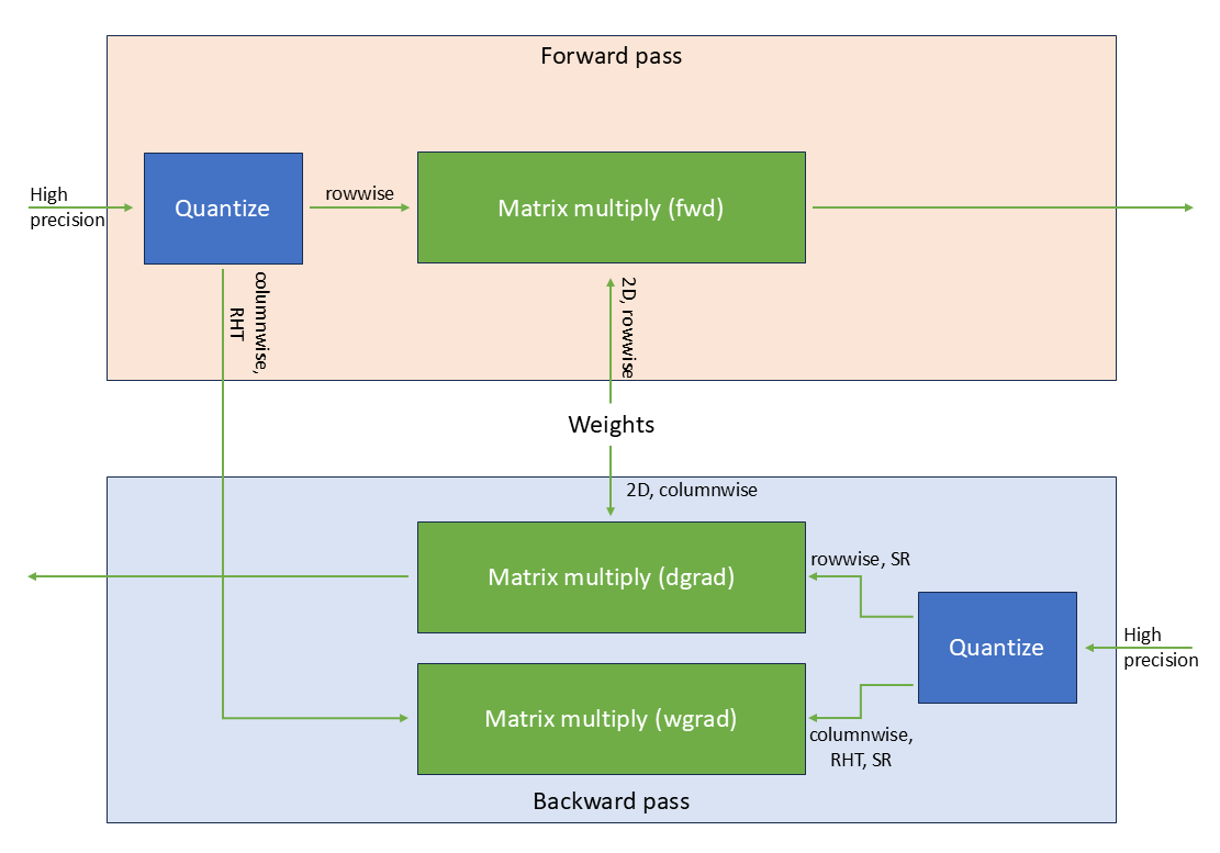
Figure 9: Linear layer utilizing NVFP4
Using FP8 and FP4 with Transformer Engine
Transformer Engine library provides tools enabling easy to use training with FP8 and FP4 datatypes using different strategies.
FP8 recipe
Transformer Engine defines a range of different low precision recipes to choose from in the transformer_engine.common.recipe module.
The DelayedScaling recipe stores all of the required options for training with FP8 delayed scaling: length of the amax history to use for scaling factor computation, FP8 data format, etc.
Float8CurrentScaling recipe enables current per-tensor scaling with FP8.
Float8BlockScaling recipe enables block scaling with FP8 as described in DeepSeek-v3 paper.
MXFP8BlockScaling recipe enables MXFP8 training.
NVFP4BlockScaling recipe enables NVFP4 training.
[1]:
from transformer_engine.common.recipe import Format, DelayedScaling, MXFP8BlockScaling, NVFP4BlockScaling

fp8_format = Format.HYBRID  # E4M3 during forward pass, E5M2 during backward pass
fp8_recipe = DelayedScaling(fp8_format=fp8_format, amax_history_len=16, amax_compute_algo="max")
mxfp8_format = Format.E4M3  # E4M3 used everywhere
mxfp8_recipe = MXFP8BlockScaling(fp8_format=mxfp8_format)
nvfp4_recipe = NVFP4BlockScaling()
This recipe is then used to configure the low precision training.
FP8 autocasting
Not every operation is safe to be performed using FP8. All of the modules provided by Transformer Engine library were designed to provide maximum performance benefit from FP8 datatype while maintaining accuracy. In order to enable FP8 operations, TE modules need to be wrapped inside the autocast context manager.
[2]:
import transformer_engine.pytorch as te
import torch

torch.manual_seed(12345)

my_linear = te.Linear(768, 768, bias=True)

inp = torch.rand((1024, 768)).cuda()

with te.autocast(enabled=True, recipe=fp8_recipe):
    out_fp8 = my_linear(inp)
The autocast context manager hides the complexity of handling FP8:
All FP8-safe operations have their inputs cast to FP8
Amax history is updated
New scaling factors are computed and ready for the next iteration
Note
Support for FP8 in the Linear layer of Transformer Engine is currently limited to tensors with shapes where both dimensions are divisible by 16. In terms of the input to the full Transformer network, this typically requires padding sequence length to be multiple of 16.
Handling backward pass
When a model is run inside the autocast region, especially in multi-GPU training, some communication is required in order to synchronize the scaling factors and amax history. In order to perform that communication without introducing much overhead, autocast context manager aggregates the tensors before performing the communication.
Due to this aggregation the backward call needs to happen outside of the autocast context manager. It has no impact on the computation precision - the precision of the backward pass is determined by the precision of the forward pass.
[3]:
loss_fp8 = out_fp8.mean()

loss_fp8.backward()  # This backward pass uses FP8, since out_fp8 was calculated inside autocast

out_fp32 = my_linear(inp)
loss_fp32 = out_fp32.mean()
loss_fp32.backward()  # This backward pass does not use FP8, since out_fp32 was calculated outside autocast
Precision
If we compare the results of the FP32 and FP8 execution, we will see that they are relatively close, but different:
[4]:
out_fp8
[4]:
tensor([[ 0.2276,  0.2629,  0.3000,  ...,  0.1297, -0.3702,  0.1807],
        [-0.0963, -0.3724,  0.1717,  ..., -0.1250, -0.8501, -0.1669],
        [ 0.4526,  0.3479,  0.5976,  ...,  0.1685, -0.8864, -0.1977],
        ...,
        [ 0.1698,  0.6062,  0.0385,  ...,  0.4038, -0.4564,  0.0143],
        [ 0.0679,  0.2947,  0.2750,  ..., -0.3271, -0.4990,  0.1198],
        [ 0.1865,  0.2353,  0.9170,  ...,  0.0673, -0.5567,  0.1246]],
       device='cuda:0', grad_fn=<_LinearBackward>)
[5]:
out_fp32
[5]:
tensor([[ 0.2373,  0.2674,  0.2980,  ...,  0.1134, -0.3661,  0.1650],
        [-0.0767, -0.3778,  0.1862,  ..., -0.1370, -0.8448, -0.1770],
        [ 0.4615,  0.3593,  0.5813,  ...,  0.1696, -0.8826, -0.1826],
        ...,
        [ 0.1914,  0.6038,  0.0382,  ...,  0.4049, -0.4729,  0.0118],
        [ 0.0864,  0.2895,  0.2719,  ..., -0.3337, -0.4922,  0.1240],
        [ 0.2019,  0.2275,  0.9027,  ...,  0.0706, -0.5481,  0.1356]],
       device='cuda:0', grad_fn=<_LinearBackward>)
That happens because in the FP8 case both the input and weights are cast to FP8 before the computation. We can see this if instead of the original inputs we use the inputs representable in FP8 (using a function defined in quickstart_utils.py):
[6]:
from quickstart_utils import cast_to_representable

inp_representable = cast_to_representable(inp)
my_linear.weight.data = cast_to_representable(my_linear.weight.data)

out_fp32_representable = my_linear(inp_representable)

print(out_fp32_representable)
tensor([[ 0.2276,  0.2629,  0.3000,  ...,  0.1297, -0.3702,  0.1807],
        [-0.0963, -0.3724,  0.1717,  ..., -0.1250, -0.8501, -0.1669],
        [ 0.4526,  0.3479,  0.5976,  ...,  0.1685, -0.8864, -0.1977],
        ...,
        [ 0.1698,  0.6062,  0.0385,  ...,  0.4038, -0.4564,  0.0143],
        [ 0.0679,  0.2947,  0.2750,  ..., -0.3271, -0.4990,  0.1198],
        [ 0.1865,  0.2353,  0.9170,  ...,  0.0673, -0.5567,  0.1246]],
       device='cuda:0', grad_fn=<_LinearBackward>)
This time the difference is really small:
[7]:
out_fp8 - out_fp32_representable
[7]:
tensor([[0., 0., 0.,  ..., 0., 0., 0.],
        [0., 0., 0.,  ..., 0., 0., 0.],
        [0., 0., 0.,  ..., 0., 0., 0.],
        ...,
        [0., 0., 0.,  ..., 0., 0., 0.],
        [0., 0., 0.,  ..., 0., 0., 0.],
        [0., 0., 0.,  ..., 0., 0., 0.]], device='cuda:0',
       grad_fn=<SubBackward0>)
The differences in result coming from FP8 execution do not matter during the training process, but it is good to understand them, e.g. during debugging the model.
Using multiple recipes in the same training run
Sometimes it is desirable to use multiple recipes in the same training run. An example of this is the NVFP4 training, where a few layers at the end of the training should be run in higher precision. This can be achieved by using multiple autocasts, either completely separately or in a nested way (this could be useful when e.g. we want to have a configurable overarching recipe but still hardcode a different recipe for some pieces of the network).
[8]:
my_linear1 = te.Linear(768, 768).bfloat16()  # The first linear - we want to run it in FP4
my_linear2 = te.Linear(768, 768).bfloat16()  # The second linear - we want to run it in MXFP8

inp = inp.bfloat16()

with te.autocast(recipe=nvfp4_recipe):
    y = my_linear1(inp)
    with te.autocast(recipe=mxfp8_recipe):
        out = my_linear2(y)

print(out)

out.mean().backward()
tensor([[ 0.0547,  0.0039, -0.0664,  ..., -0.2061,  0.2344, -0.3223],
        [ 0.0131, -0.1436,  0.0168,  ..., -0.4258,  0.1562, -0.0371],
        [ 0.1074, -0.2773,  0.0576,  ..., -0.2070,  0.0640, -0.1611],
        ...,
        [ 0.0825, -0.0630,  0.0571,  ..., -0.3711,  0.1562, -0.4062],
        [-0.1729, -0.1138, -0.0620,  ..., -0.4238,  0.0703, -0.2070],
        [-0.0908, -0.2148,  0.2676,  ..., -0.4551,  0.1836, -0.4551]],
       device='cuda:0', dtype=torch.bfloat16, grad_fn=<_LinearBackward>)