Overview
Deep learning models consist of many layers of processing, arranged as a computation graph, where the output from one layer serves as input to subsequent layers. The post-layer tensor data for input processed through a given layer is also known as that layer’s feature map since it represents the features extracted by the network when input data has flowed to that point in the computation graph.
Feature maps are typically tensors having large channel counts, and the same number of batch items as the original input. Understanding the information found inside the feature maps of a network model provides a lot of information about the effectiveness and potential deficiencies of that model, while also providing clues about how the model (or related training parameters) can be optimized to get better inference results.
What Does Feature Map Explorer Do?
Feature Map Explorer (FME) enables visualization of 4-dimensional image-based feature map data in a fluid, interactive fashion, from a range of summary views, to low-level channel visualizations, to providing detailed numerical information about each channel slice. Think of this as a way to peer into the DL processing “black box” to find intimate information about what the model is learning, where the model is failing to use resources efficiently, and what is changing as a model is learning during training to better process data handed to it.
Why is this Useful?
By providing a fast way to visually inspect the processing taking place across the layers of a DL model, the DL developer is efficiently informed about where the model is performing well and where it is falling short. This, in turn, can be used to help guide changes to the model architecture or to other training-time parameters in order to improve overall quality. In this manner, FME is similar to a traditional code debugger, where the ability to inspect runtime state is a valuable tool in any developer’s toolbox.
Exploring feature maps is not a new concept, but FME takes what used to be a slow, tedious process and makes it fast and efficient by leveraging GPU processing to visualize what is contained in the large feature map tensors. By allowing for fast exploration of feature maps from a large number of layers, across batch items and training epochs, FME can raise developer productivity during both the initial model design phase as well as during subsequent tuning phases.
General Familiarity
In this section, we’ll cover the use of Feature Map Explorer in high-level form so you can get started reasonably quickly. Later, we’ll cover additional topics in greater detail.
UI Layout and Terminology
The FME UI consists of a central viewing region as well as panels whose layout positions can be rearranged by the user. Reconfiguring the UI consists of dragging panels and/or separators in standard fashion so we won’t go into details about that process here.
The main areas of the UI consist of the components described below. These brief descriptions serve just to summarize major functionality. More detailed information is provided in the remainder of this document.
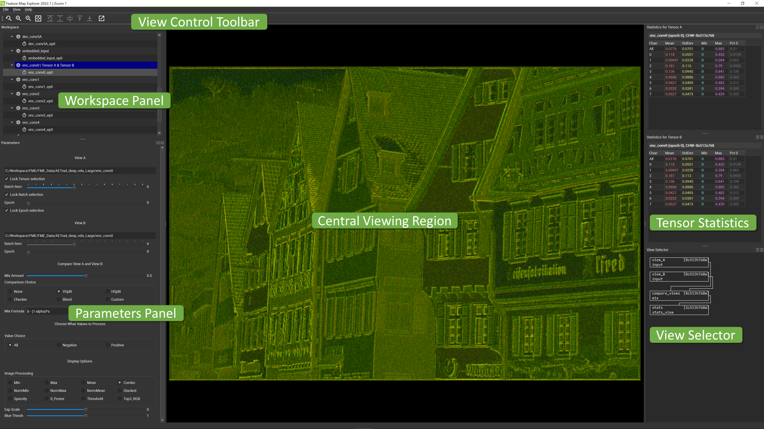
- Central Viewing Region: Location of graphical summary and detailed channel views for the selected feature map.
- Workspace Panel: List of available feature maps tensors to quickly call up for viewing on demand.
- Parameters Panel: Main controls used to select which batch item and epoch is currently being view, as well as how summary views are processed to extract information.
- Tensor Statistics: Detailed information regarding the contents of the selected feature map tensor (for the specified batch item and epoch).
- View Selector: Control of Summary View or Channel View for the central viewing region.
- View Control Toolbar: Action buttons to control view scaling in both the spatial and color dimensions.
High-level Workflow
- Load feature map directories into the workspace. An individual feature map is selected for viewing and analysis solely from the Workspace panel.
- Select a feature map from the workspace and observe summary views and per-channel visualizations in the central viewing region. Control of parameters of the summary view is made in the Parameters panel, and toggling between summary and channel views is made in the View Selector panel.
- Explore the data in your selected feature map by trying out different processing methods for the summary view using the display options available in the Parameters panel. Because feature map tensors typically have a large number of channels, reducing the information to a simple visual form requires extracting and reducing the information in a tensor with 3 or fewer channels for visual display. The types of extraction and reduction methods vary in their ability to bring out or hide information in the large amount of feature map data.
- Explore all of the feature map tensors in your model (which is often best to do in the order your original model processes the data) and look for trends or anomalies that are unexpected and/or unwanted.
- Note that you can also vary which batch item you are visualizing (so you can easily explore your model with varying input values from within a single FME session), and if you have feature maps generated from the same input batch across multiple training epochs, you can move the epoch slider while exploring a fixed tensor to see how the network evolved its processing of that data during training.
Note that this workflow is largely exploratory, as opposed to always following a fixed set of well-defined and well-ordered steps. The key to gaining insight into what your model is actually doing when processing a batch of input is to interactively explore the feature map transformations, vertically as data flows through the model (from layer to subsequent layer), and horizontally by varying the batch item processed at a particular layer.
For example, if you see places where valuable information disappears from the feature maps as you move from one layer to the next, this would warrant further study of your model or training data and methods to find out why the model was losing information during training. Or, if you see that similar features are extracted (or ignored) when varying the batch item processed at a particular layer, this may indicate that your model is not distinguishing features that you may deem valuable, hence leading to an overall loss of quality.
Get Started
We will now walk through how to use FME in a bit more detail.
How are Feature Maps Obtained?
Not surprisingly, in order to use Feature Map Explorer, you will need to generate some feature maps from your trained model. This is a straightforward task with most training frameworks, since FME directly consumes feature map tensors written out as standard numpy array files (i.e. the .npy files written by the np.save() method). These files are assumed to contain 32-bit single precision floating point values in a 4D array with order NCHW (where N is the batch size, C is the channel count, and H and W are height and width respectively). If your training data is in NHWC (channels last) layout, you will need to transpose the axes (e.g. permute the axes with a (0,3,1,2) permutation) before calling np.save().
As you process a single batch of input, you should save feature maps for all the layers you want to investigate into a single directory. For ease of exploration within FME, the names of saved .npy files should reflect the identities of the layers that generated those feature maps since the name of the .npy file will be the only identifier that shows up in the FME UI.
With this in mind, please note that the feature map file names (as supplied by you to the np.save() method) have to follow a specific format: For example, if you have a model with a layer called “conv1”, you should save the feature map tensor in a file called “conv1_ep0.npy”. And if you want to represent hierarchies or blocks of layers, we suggest the use of the underscore character as a separator (e.g. “resblock1_conv1_ep0.npy” and “resblock2_conv1_ep0.npy”).
More detailed info: If you want to explore how feature maps evolve during training (by saving feature maps obtained from a fixed batch of data processed across multiple epochs), you should write the feature maps into a single directory (as above) using names like “ID_epN.npy” where ID is the identifier for the layer producing this particular feature map and N is the epoch number after which you are writing out the feature maps. For example, “conv1_ep12.npy” would be a good name choice for the feature map coming from layer “conv1” after epoch 12. (Note: You do not need to write out feature maps for every training epoch. And if you only want to write out feature maps for a single epoch or only after training is finished, the epoch number can be anything you want as long as each .npy file name uses the same number. The “_ep0” suffix suggested above is just a standard convention.) Also of note: If you want to investigate feature maps for multiple batches of input data, you should save the feature maps generated using each batch into a separate directory since FME will assume all tensors in the same directory were generated by the exact same single batch of input.
Loading Feature Maps
- Use the menu choice File | Add Tensor NPY Directory and browse
- Use the hotkey combination of Control+W and browse
- Drag the NPY folder to the Workspace Panel in the UI
When you select a directory, FME will scan and display the names of the tensor files it found in an expandable list in the workspace panel. The hierarchy is: Directory Name : Base Tensor Name : Individual Tensors (per epoch).
Each time you load a directory of .npy files into the workspace (and you can add as many directories as you want), the list of added tensors starts out fully expanded so you can see explicitly which files were found. That said, it is often most useful to collapse the actual file names since typically selection is done at the Base Tensor Name level. To collapse the individual names, you can right click on the Directory Name and select Inverse Expand, or you can simply double-click on the Directory Name. (Both of these actions are toggles.)
To collapse the Base Tensor Name lists, click on the down arrow to the left of the name (and click again on the same area, which now shows a right arrow in order to re-expand the list).
Note: To remove a directory from display in the workspace, right-click on the top level directory name and choose Remove. This is non-destructive (in that the files will still remain on disk), so you can add this directory back into the workspace later, if desired.
Viewing a Feature Map
A key step in exploring your network model (through the lens of feature map visualization) is the ability to rapidly select a tensor for visualization. This is why the Workspace panel exists (as opposed to having a File | Load NPY File menu option for individual feature map files): By showing all of your feature maps grouped by directory (and thereby associated with a single input batch) in a list, you can simply double-click on the Base Tensor Name (which is the most common approach) or you can double-click or right-click an Individual Tensor Name (per epoch) to select that tensor for visual processing.
Note: If you select an individual tensor, the epoch being viewed will also be updated to match the epoch in your tensor selection (by parsing the number after “_ep” in the tensor name). If you select a tensor using the Base Tensor Name, the epoch slider will not move from its current position. You can also load a tensor for viewing by right-clicking on its name (at the base name or individual name level) and choosing the appropriate Select menu item.
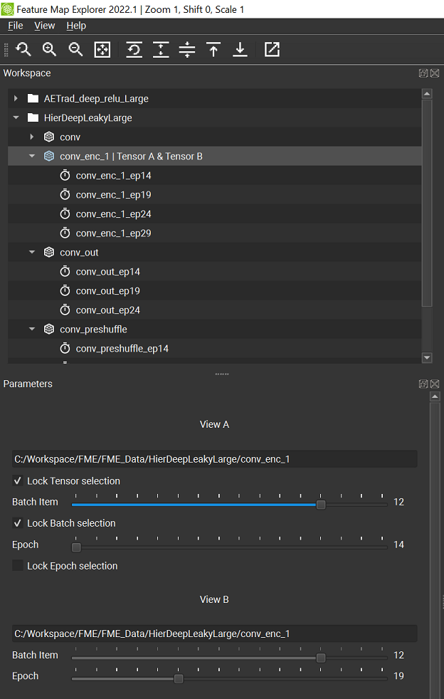
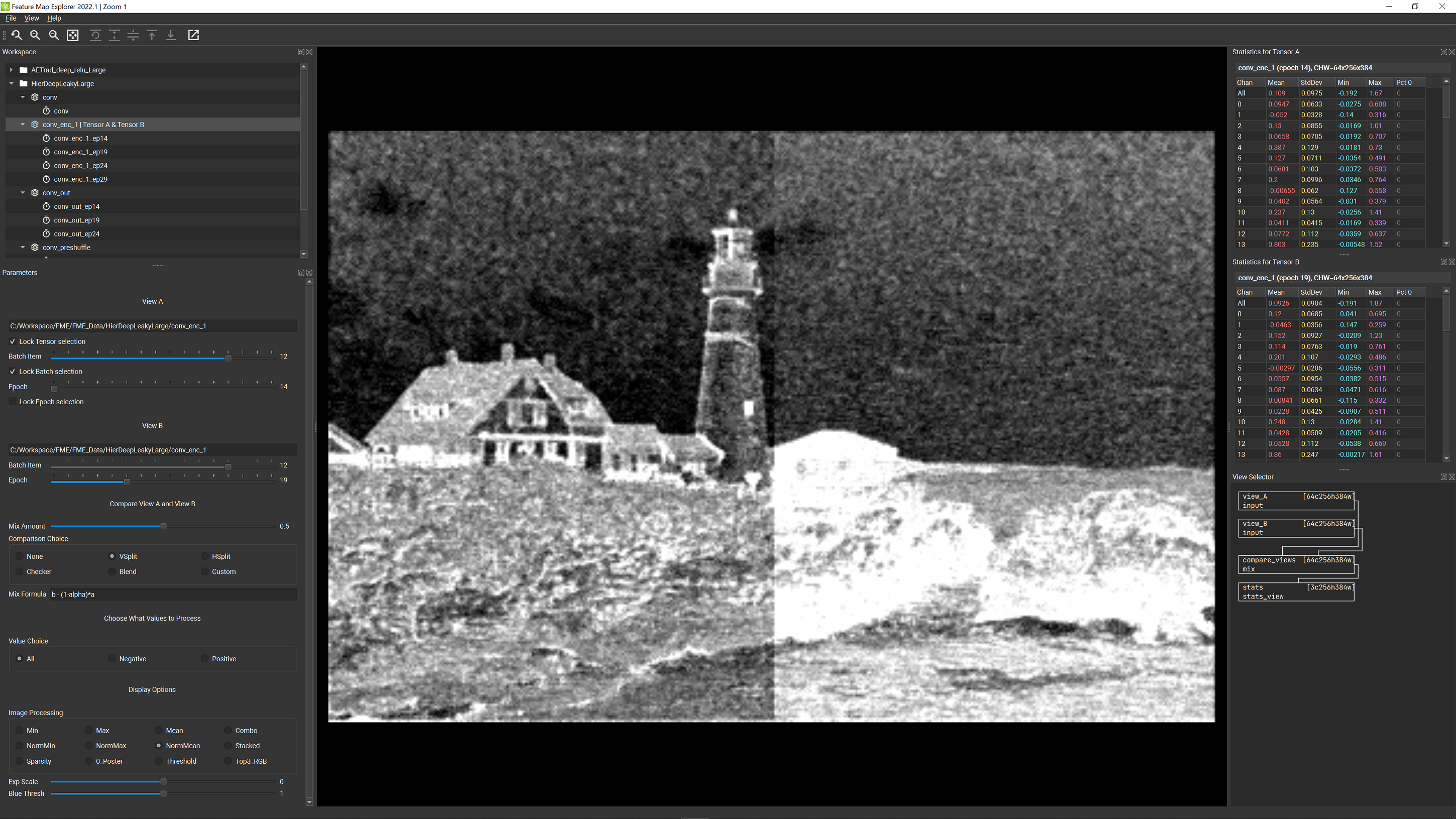
Terminology: FME actually allows you to select two separate tensors (marked as Tensor A and Tensor B in the Workspace panel) at once, and visualize them from two different views: View A and View B (defined under the View A and View B sections of the Parameter panel, and switchable from the View Selector panel) respectively. By default, these two tensor choices are locked to the same selection (via the Lock Tensor slection checkbox in the View A section of the Parameters panel), but you can still having two different views by varying the Batch Item slider or the Epoch slider (the Lock Batch selection and Lock Epoch selection checkboxes in the View A section of the Parameters panel need to be unchecked). See the following screenshot for an example of selecting tensor conv_enc_1 from epoch 14 for view A and the same tensor from epoc 19 for view B.
If you want to compare two completely different feature map tensors (say, one coming from your training framework and one coming from some low-level code you wrote for inference), you can unlock the tensor selections (by unchecking the Lock Tensor Slection checkbox) and explicitly load separate tensors into View A and View B.
In this Getting Started section, however we’ll assume that the tensor selection is locked, and we will address more advanced uses of unlocked tensor selection later.
Summary Views
Once you double-click a tensor name in the Workspace list for viewing, the Center Viewing Region will display a summary view of the feature map contents (note: Summary View is shown only when nothing is selected in the View Selector panel). This is actually a view of a 3D slice of the full 4D feature map tensor: It has dimensions CHW and is extracted from the full NCHW tensor by setting N to the batch item number currently selected on the Batch Item slider located near the top of the Parameters panel.
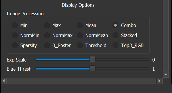
There are many different types of summary views, and they are selected by use of the twelve radio buttons in the Image Processing section at the bottom of the Parameters panel.
Getting familiar with the various types of processing options will be time well spent, but first we should describe why there are so many options: The key problem is that feature map tensors will typically have a large number of channels, but a visual representation only has three channels (red, green, and blue) available for displaying the summary. Thus, in order to present information contained in a high-channel-count tensor, it is necessary to do some sort of image processing to condense the tensor’s channel-rich information into a viewable form.
- An array of mean (i.e. average) values across all the channels at each horizontal (x) and vertical (y) location in the CHW tensor slice is computed. This array is of size HxW.
- The mean and standard deviation of the above array is computed. These are scalars.
- The RGB values being displayed come from subtracting the scalar mean from the array of “per-pixel” means and then scaling the result across 3 standard-deviations. By scaling, we mean that values 3 standard deviations or more below the overall mean are displayed as black, and values 3 standard deviations or above the overall mean are displayed as white, with values in between ranging linearly from black to white.
That’s a mouthful to describe, but in general the visual effect is to accentuate features independent of the actual range of values in a given tensor. Note that the processing choices are designed with (potentially) revealing structure as their main goal, not a detailed numerical analysis of the feature map slice.
Note: If you are curious about the actual numerical ranges, you can check out the Statistics panel (available for either Tensor A or Tensor B, but in our case these will show identical information since we’ve locked the tensor selection so A and B are the same). The statistics displayed there include the min, max, mean, and standard deviation values for the overall CHW tensor slice, as well as that same set of values for each individual value channel slice.
In similar fashion, NormMax computes the “per-pixel” maximums across all channels, then finds the mean and standard deviation of those maximum values, and scales the resulting display by 3 standard deviations centered about the mean. And NormMin works similarly.
Go ahead and try this out, and also feel free to move the Batch Item slider at any time to see how these views differ for the various input batch items you used during creation of your feature maps.
In general, NormMean tends to show the “mainstream” features well (since the mean is typically a reasonable proxy for the all the channel values at a fixed (x,y) position), whereas NormMax and NormMin tend to expose “outlier” features.
Note: If you are looking at feature maps saved right after ReLU activation, the NormMin display will (usually) be all black. This is because at least one channel in the feature map tensor will likely have a 0 value at any given x,y location, so the min array will be all zeros.
As interesting as it may be to look at NormMean, NormMax, and NormMin summaries, because of the extreme data reduction involved in computing means, maximums, and minimums, it is possible for these summaries to be misleading. For example, in the case where one channel in the feature map is the exact negative of another, those two channels will completely negate each other when computing these summaries, and hence any information they may hold will disappear from the visual display.
Introducing Channel Views
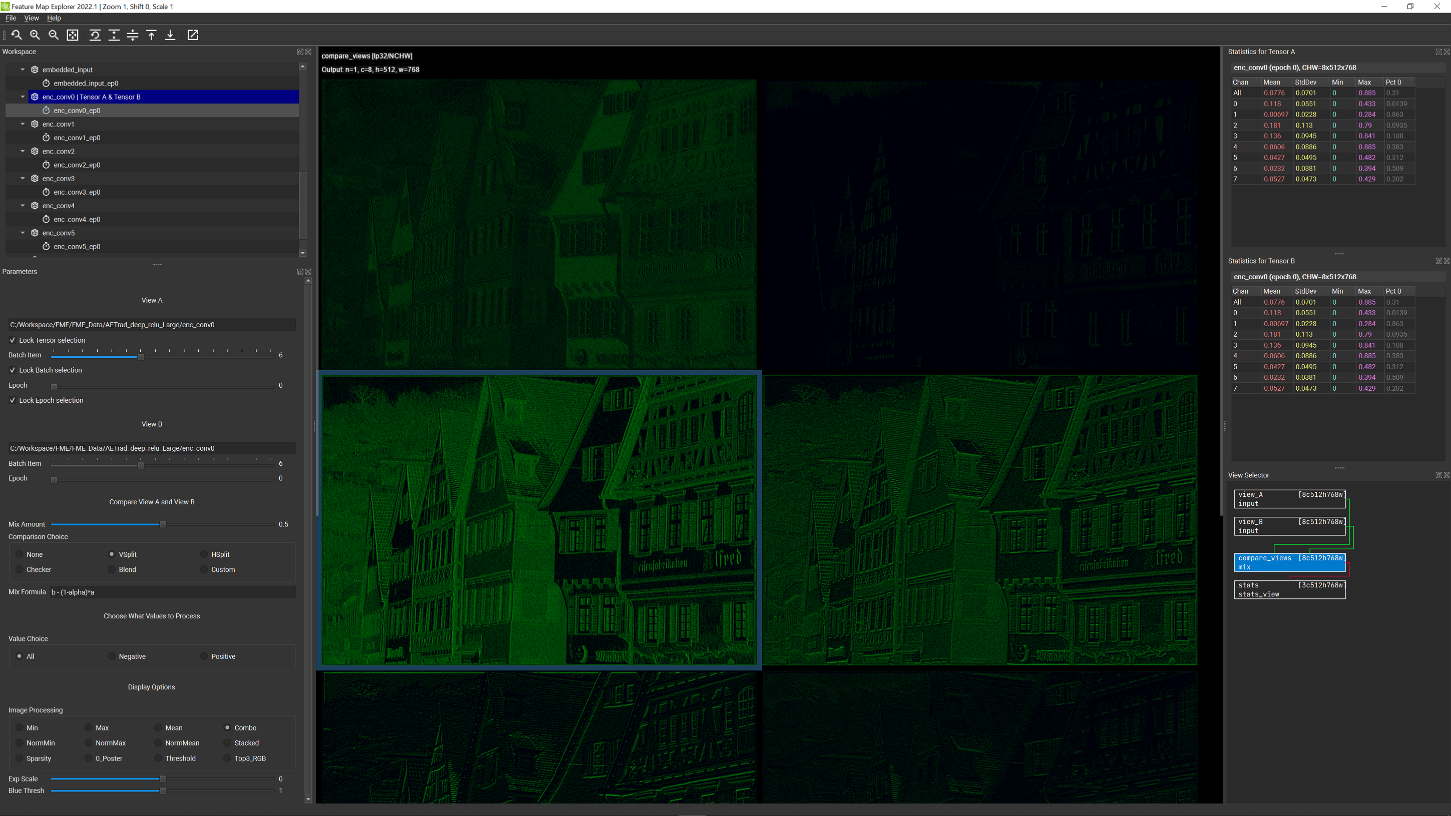
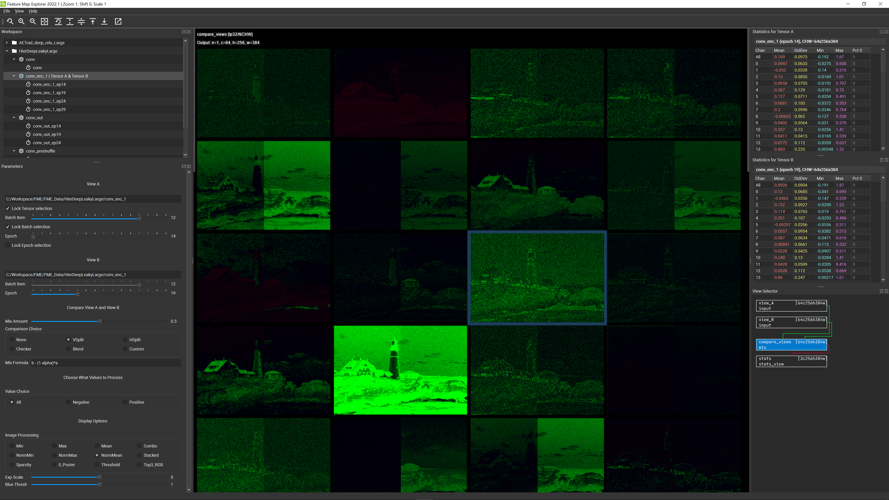
In case this makes you feel a bit queasy, please be assured that you also have the ability to see all of the unprocessed data too! This is possible through use of the View Selector panel. We’ll have more to say later about why there are four choices in that panel, but for now, if you click on the box labeled compare_views you will see a display consisting of a grid of C (channel count) rectangles of size HxW. These HxW rectangles are visualizations of each of the C channel slices in the current feature map tensor (for the selected batch item, which, as always you can change at any time using the Batch Item slider).
The channel display shows positive values in green and negative values in red. Brighter values indicate higher magnitudes and values closer to black indicate lower magnitudes.
Since the overall range of values can vary dramatically from one feature map to the next, FME automatically scales the color range by the overall extremes so that if something is there (for at least one channel), it shows up. This automatic color-range scaling is usually useful, but of course you can turn it off if you don’t want to use it (via the View | Auto Scale Channels menu item or the Ctrl-Shift-C hotkey combo).
Navigation of the Central Viewing Region
This is also a good place to talk about navigation options for the Central Viewing Region.
Since there can be a large number of channel slice rectangles they are unlikely to all fit in their viewing region at once. To scroll others into view, you can either click-and-drag (up and down) or use the wheel on your mouse. Or, to see more (or fewer) of the channel slices at once, you can hold down the Ctrl key while using the mouse wheel. This will shrink or enlarge the displayed size of the rectangles.
Note: The buttons on the left of the top toolbar offer another way to control image size. The magnifying glass buttons use should be obvious. The fourth button is a toggle to turn on/off discrete zoom as a way to force the displayed channel slices to be “pixel accurate”.
You can also use the Alt-wheel and Shift-wheel combinations to scale or offset the displayed color values, or use the toolbar buttons on the right of the toolbar to achieve these same actions.
Before returning to discuss more Summary View options, we’ll show you one more fun feature with channel value viewing: It often turns out that the magnitudes of the minimum and maximum tensor values are significantly different. (For example, if you use Leaky ReLU activation, the negative values tend to be multiplied by 0.1 whereas the positive values are not changed.) This means that it is not uncommon for the features captured in the negative (red) values to be visually dwarfed by the features captures in the positive (green) values. Put simply, the red values often disappear in a sea of green.
To overcome this, we offer filtering options in the Value Choice section of the Parameters panel that limit the displayed values to either those that are negative or those that are positive. And because the channel view will auto-scale color ranges, jumping between the All, Negative, and Positive in the Value Choice section will consistently scale the visual display appropriately.
Note: This only works if you have the compare_views rectangle selected in the View Selector panel. It will not work if you select either view_A or view_B. The explicit view choices display the tensor values before any processing steps, hence they aren’t affected by the Value Choice selection.
While it can be very interesting and informative to examine channel slices in detail, it can also be tedious and hard to know which features line up (or diverge) between one channel slice and another faraway slice in the display grid. And it may be difficult to get a general feel about which large features are properly detected in general, and what details may be missed. The upshot is that Summary Views and Channel Slice visualization offer complementary pros and cons, and neither alone is adequate. That is why FME makes it easy to toggle between these viewing options.
Returning to Summary Views
With this in mind, let’s return to our discussion of Summary Views.
To get back to viewing tensor summaries (rather than individual channel values), simply click on the high-lit View Selector rectangle or anywhere outside the rectangles in the View Selector panel. The rectangle will return to its unselected state, and the Central Viewing Region will return to displaying a Summary View.
By this point, you may have already forgotten what NormMean, NormMax, and NormMin do. For a quick summary, hover your mouse over any of those radio buttons and observe the brief description pop-up at the bottom of the application window (on the bottom status bar area). For example, hovering over the NormMean button will display “Normalized Mean (centered about mean, +/- 3 standard deviations)”. This is intended to serve as a quick reminder to maybe save you a trip back to this documentation.
The next group of choices we’ll describe are the Min, Max, and Mean options on the top row of the Image Processing choices. As you might guess from the brief help text, these options work similarly to their “Norm” counterparts. The difference is that instead of normalizing the displayed ranges based on mean and standard deviation, the Min, Max, and Mean options always scale the Summary View to show black at the overall min value, white at the overall max value, and gray in between. In particular, this means that at least one pixel will be true black in the Min view, and at least one pixel will be pure white in the Max view. But because the minimum and maximum values may be outliers present on just one channel slice, these views tend to appear more “muted” (i.e. more dominantly gray) than their “Norm” counterparts.
Note: Having the ability to vary the intensity range in Channel View was a useful option and for muted displays in the Summary View, it may also be useful to be able to exaggerate (or diminish) displayed ranges. This can be accomplished by using the Exp Scale (exponential scale) slider near the bottom of the Parameter Panel. Moving the slider to the right of center scales up the feature map tensor values (and tends to make summary images brighter), whereas moving the slider to the left of center scales down the values, and tends to darken summary images. To turn off value scaling, return the slider to the center by double-clicking on the “Exp Scale” label. (For future reference, this double-click-on-the-label trick will also work to center the thumb on the Mix Amount and Blue Thresh sliders.)
To wrap up this section, we’ll describe three of the remaining 6 Image Processing choices:
- Combo produces a pseudo-color RGB summary where the maximum values are displayed in the red (R) channel, the mean is display in the green (G) channel, and the minimum is displayed in the blue (B) channel. This display helps draw your eyes to places where the correlations between the min and max values vary.
- Stacked follows a similar convention to the channel slice views, where green represents positive values and red represents negative values, with intensity tied to magnitude. But in Summary form, the channel values are averaged for each (x,y) position. This is a significant reduction of detailed information, but it does offer a nice complement to viewing a large grid of channel slices.
- Finally, Top3_RGB offers a simple way to view feature map tensors that actually represent standard RGB images. This summary is created having the first three channels represent the red, green, and blue channels in the Summary View display, but do note that FME assumes that tensor “component color values” range from -0.5 to 0.5 (i.e. not 0 to 1), so if your network was following some other convention, or some other color space, this Summary View choice may not work as you might otherwise expect.
Wrapping Up
In addition to the remaining three Summary View choices (Sparsity, 0_Poster, and Threshold), there are still many features and capabilities in FME that we haven’t discussed yet. These mainly involve comparing two completely separate tensors or a single tensor with itself at different points in “time” (i.e. at a different training epoch). These topics are not harder than what you’ve learned so far, but they do build on what has already been presented. Thus, we recommend you play with the capabilities already described, and once you are comfortable, return to this document to learn more about what else FME offers.
Going Further
In the Getting Started section we covered a range of options for visualizing individual feature maps, using various summary views or by way separate channel slices. By using the batch item slider to see what varies as input value change, or by tracing the flow of data through the network by manually selecting successive layers in your model for visualization, it is possible to get a better feel for how your model is processing data.
The key here is that observing changes (by varying batch item or model layer) provides insight that complements and extends the information available from static analysis of an single feature map. Feature Map Explorer extends the ability to visualize changes by allowing you to see how feature maps evolve as training progress.
Assumptions
- The same input batch of data is processed at each epoch of interest in order to produce consistent feature maps. This is required in order to see how the processing of that fixed data evolves while training progresses.
- Feature maps are written out using file names of the form “tensor_name_epN.npy”, where tensor_name is a string of your choosing (though we recommend avoiding dashes and spaces) and N is the epoch number associated with that feature map. So, for a layer called “conv1” trained over 10 epochs, names like “conv1_ep0.npy, conv1_ep1.npy, conv1_ep2.npy, …, conv1_ep9.npy” would be reasonable.
- There is no need to write out data after each epoch. For example, you may want to write feature maps out only after every 10th epoch has been trained. In the FME UI, if you set the slider to an epoch number that has no associated feature map file, FME will iteratively reduce the epoch number used in its file name search until it finds a match. (This allows for “scrubbing” the epoch slider and seeing smooth evolution, even if data for some epoch numbers is missing.)
Note: Tensor Statistics are only displayed for the currently selected epoch without any under-the-covers adjustments. This means that if the Epoch slider is set to an epoch number for which there is no corresponding feature map file available, the associated tensor statistics window will be empty.
Comparing Feature Maps Across Epochs
When you load a folder containing feature maps that span multiple epochs, and select one of those feature maps, each of the two Epoch sliders (one for View A and one for View B) in the Parameters panel are redrawn to allow epoch selection from the minimum to the maximum epoch numbers that are available.
By selecting two different epochs for View A and View B, you can then make comparisons by choosing an option in the Comparison Choice box. Here is a summary of the options available:
- None: Just display View A all the time. View B is ignored
- VSplit: Split the view vertically, between View A and View B, where the location of the vertical split is controlled by the Mix Amount slider at the top of the Compare View A and View B section. View A is shown to the right of the split and View B is shown to the left.
- HSplit: Similar the VSplit, but in this case the comparison boundary is horizontal. View A is shown below the split, and View B appears above the split.
- Checker: Use the Mix Amount slider to control the size of a checkerboard where alternate tiles show View A and View B
- Blend: Move from displaying View A only, when the slider is fully to the left, to View B only, when the slider is fully to the right. For intermediate positions, a linear interpolation of View A and View B is displayed.
- Custom: This option allows you to use a custom comparison formula that you supply yourself. Inside a formula, a represents View A, b represents View B, and alpha represents the position of the Mix Amount slider (with 0 meaning fully to the left, 1 meaning fully to the right, and intermediate values moving proportionately from 0 to 1 as the slider moves to the left).
Note: The Custom formula provided by default, b-(1-alpha)*a, calculates the difference between View B and View A when the slider is fully to the left (where alpha is 0), and displays View B only when the slider is fully to the right (and alpha equals 1). It is possible to use most math expressions (including trig functions like sin and cos, transcendental functions like log and exp, and operators like +,-,*,/,^) in custom formulae.
Summary View Order of Processing
The following screenshot shows the comparsion of the same tensor across two different epochs in the summary view:
When comparing feature maps using Summary View (using any of the comparison choices), the Image Processing formulas apply to the current comparison view (e.g. the maximum, minimums, means, and standard deviations used in the various formulas are calculated for the composite view with possibly A and B both present). For this reason, you may see some noticeable range shifts taking place as you move the mix slider. This is especially true if View A and View B are distinctly different (which may happen if training is failing to converge, or you are comparing a feature map produced early in training with another produced much later).
Comparing Tensors using Channel View
You can also visualize comparisons directly with the Channel View option. If you toggle on compare_views in the View Selector, the channel slices will be shown with results after the current Comparison Choice is applied. If you want to see raw channel data, switching from the channel view to view_A or view_B will display the unprocessed channel slices for tensor A or tensor B. (Note: if you want to use a fixed color range for channel visualization, you should use the View | Auto Scale Channels menu item to toggle automatic channel scaling off.)
Visualizing Training Progress with Summary Views
Often, training progress is measured and reported using the value of the composite loss function used during training, or a small set constituent values contributing to the overall loss. This is usually a good way to summarize training progress or compare the convergence of different training scenarios. But it fails to provide any detailed information about the circumstances under which the network does well or runs into trouble.
This is where FME can help provide some insight. If you choose Custom from Comparison Choice, leave the Mix Formula at its default value with the Mix Amount slider at 0 (far left), or change the Mix Formula to simply b-a (which makes the comparison independent of the Mix Amount slider position), FME will show you the difference between views A and B.
This means that if you set the epoch slider for View B at the last trained epoch, and then scrub the epoch slider for View A from the first available epoch over to the last, you will see the how the training converged to the final state (at least for the particular input and batch item being viewed).
However, there is a big downside to the way FME presents this information when using the Image Processing options popular in the Getting Started section: Recall that these options were designed to “draw out” the features present in a feature map with large channel count, by scaling even small differences to broader monochrome or color ranges? Well, this processing still takes place even when you are viewing differences – so small differences become more exaggerated the closer View A is to View B. There are circumstances when this could provide some insight, but generally speaking, it is not very satisfying to expect to mainly see convergence but instead see overly-emphasized differences.
The Threshold option from Image Processing is offered to address this problem. It works by displaying areas that are close to zero in blue, with red and green values of varying intensity used for negative and positive values just like when using the channel view.
With Threshold chosen, you have the ability to control how close to zero the values have to be (in absolute value) before they are colored blue. This is done by moving the Blue Thresh (old) slider. The threshold gets smaller as the slider is move to the left (down to 0) and higher as the slider is moved to the right.
Settings for the Blue Thresh slider only come into play when the Threshold Image Processing choice is active. However, the Exp Scale slider directly above it is always active and can be useful whenever feature map values have ranges that could benefit from manual scaling (either up, or down).
Exp Scale is short for "Exponential Scaling”, with the label chosen to describe the scale factor produced by moving the slider: When the slider is in the middle, with value zero, the values in feature maps are scaled by 10^0 (which equals 1, so there is essentially no scaling). When the slider is moved to the right, the exponent is positive so feature map ranges are expanded, and when the slider is moved to the left, the exponent becomes negative which in turn means feature map ranges get compressed.
The key point here is that the Exp Scale and Blue Thresh sliders can be used together to emphasize (or diminish) differences shown between Views A and B when the Threshold Image Processing option is active.
Tip: All FME sliders can be quickly set to their midpoint by double-clicking their associated label. This is especially useful for the Exp Scaling slider, since double-clicking its label will quickly reset scaling to 1.0.
Viewing Training Progress with Channel Views
If you have multi-epoch data and want to view the differences between View A (set to one epoch) and View B (set to a different epoch), choose the Custom from Comparison Choice with a difference formula in the same way as described in the prior section.
By clicking on compare_views in the View Selector panel, you will then see channel slices of the tensor calculated as the difference between View A and View B. In this case, you will probably want to turn off auto-scaling of range values (which is the feature described in Getting Started, where FME tries to make sure full color ranges are used for quicker feature visualization).
To turn off auto-scaling of channel values, unselect the menu toggle located at View | Auto Scale Channels. Note that you can still use the top toolbar or Alt + mouse wheel to choose a fixed scaling value that allows for visually extracting the information that is of most interest to you.
Narrow Focus: Sparsity Investigations
For some deep learning problems, sparsity plays a big role (where sparsity here refers to “activation sparsity” or areas where feature maps have the value 0). The Sparsity and 0_Poster Image Processing choices are designed to visually aid in sparsity analysis. We will not dwell on these options here, since they only apply to this focused area of investigation. If you are working in this area, then the brief, on-screen summaries likely provide sufficient details about how to use these options productively.
General Tensor Comparisons
Finally, we want to point out that Feature Map Explorer can also be used as a general 4D tensor visualization and comparison tool (where these tensors are not necessarily even feature maps).
Comparison of tensors can be useful under many circumstances, such as while trying to debug why a standalone inference-only version of a fully trained network is not producing the same results as direct evaluation of the same network within the training environment.
By dumping feature maps from both the training and inference implementations (for the same fixed input, of course), corresponding pairs of feature maps can be quickly visualized (either directly, or using the comparison tools) to spot the point where internal results first start to differ.
To load disparate tensors into View A and View B, you need to uncheck the Lock Tensor selection checkbox near the top of the Parameters panel. When tensor selection is not locked, the right-click menu for tensors in the Workspace panel explicitly allows you load tensors into either View A or View B.
There is one big constraint: It is your responsibility to make sure that the tensors in View A and View B have the same dimensions if you want to use any of the nontrivial options from Comparison Choice. If the dimensions don’t match, FME will report the problem in the main viewing area.