Overview
NVIDIA Nsight Deep Learning Designer is a software tool whose goal is to speed up Deep Learning developers' workflow by providing tools to design, profile, and analyze models in an interactive manner.
Using NVIDIA Nsight Deep Learning Designer, you can iterate faster on your model by rapidly launching inference runs and profiling the layers' behavior using GPU performance counters. With the Analysis mode, you can verify the quality of your network and even inspect individual feature maps using the debugger.
NVIDIA Nsight Deep Learning Designer depends on NvNeural, its companion inference framework. To interact directly with it you can use a CLI application named ConverenceNG. Using the command line, you can launch an inference run, profile, or export your model.
To get the full list of available subcommands, use:
ConverenceNG --help
To get the list of arguments of a specific subcommand, use:
ConverenceNG <subcommand> --help
2. Model Design
Understanding how to efficiently design a model inside NVIDIA Nsight Deep Learning Designer and leverage the various features to do so is crucial.
2.1. Workspace
The central element in the NVIDIA Nsight Deep Learning Designer workspace is the canvas where you create your model graph by dropping layer nodes and connecting the nodes. The workspace can be arranged using the dockable tool windows to best fit your desired workflow. All tool windows can be found under View > Windows. Refer to the commands under the Window menu to save, apply or reset layouts.
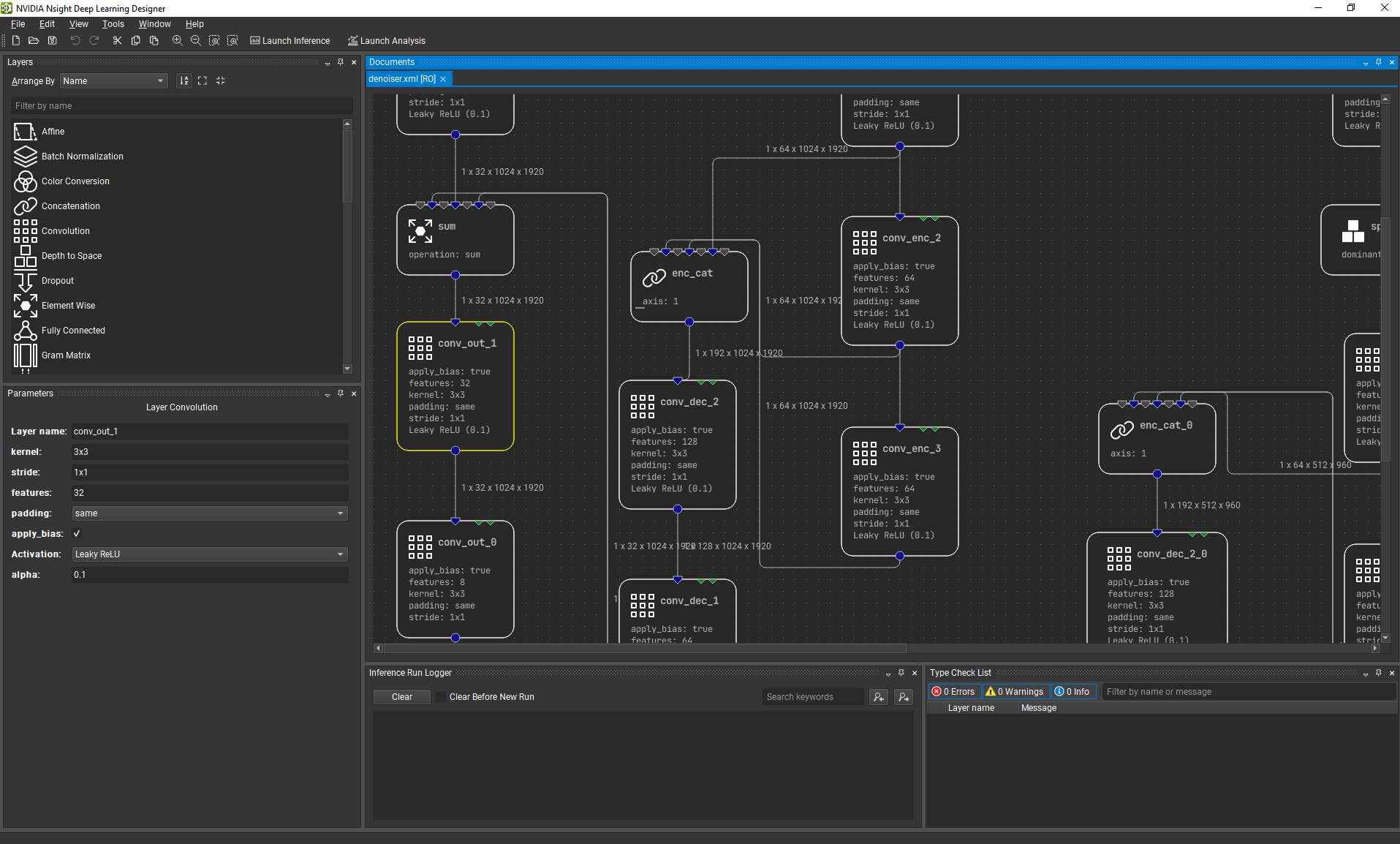
The default workspace is composed of the Layer Palette, the Parameter Window, and the Type Checking window.
Before going into the details of creating a new network, it is important to understand how individual deep learning layers are managed.
2.2. Layers
NVIDIA Nsight Deep Learning Designer aims to be modular to allow and encourage users to develop their own layer or activation implementations using the NvNeural SDK. Layers and activation functions are grouped into plugins. Any layers or activation that is used inside the application come from a loaded plugin. Even though NVIDIA Nsight Deep Learning Designer is distributed with a set of standard implemented layers and activation, you are free to unload them or load additional plugins that you have created or shared from other developers.
Using the collection manager dialog located in Tools > Manage Collections, you have access to the list of loaded plugins and their metadatas: author, description, version. Using the checkboxes, it is possible to load or unload a specific plugin:
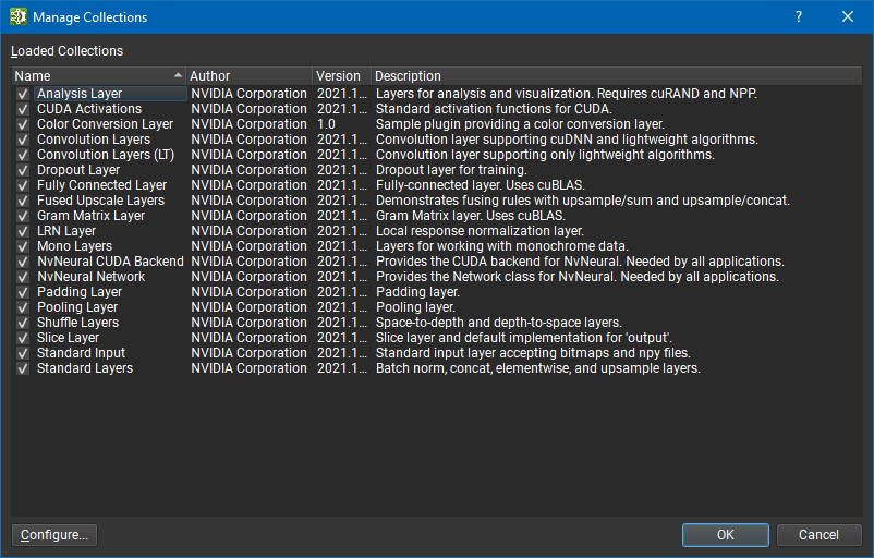
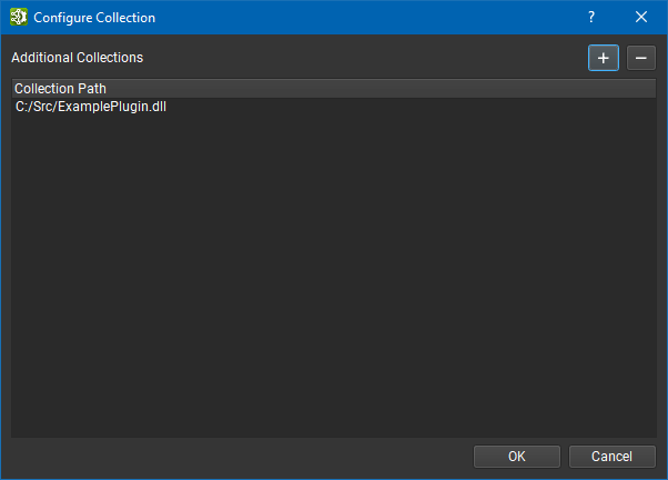
The Configure button allows you to specify additional plugins that should be added to that list. The editor preserves your selection across application launches.
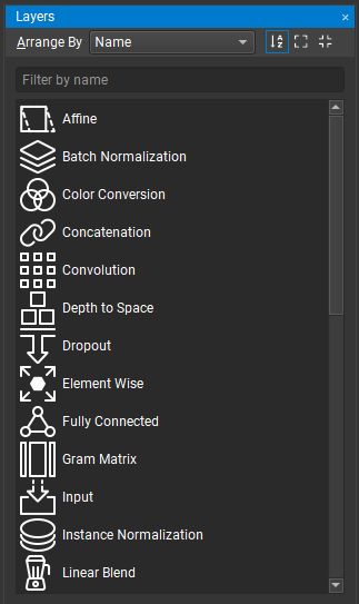
The Layer palette holds the list of available layers that can be used to design a model. These layers are gathered from the list of loaded plugins. Layers can be arranged by name, collection, or category. The Layer palette can also be sorted or filtered. To add new layer instances to the canvas, simply drag and drop from the palette.
2.3. Parameters
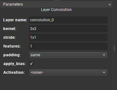
The parameter tool window allows you to interactively modify any layer’s parameters. To do so, select a layer from the canvas; available parameters for that layer will then be listed. This is also where activations can be chosen for applicable layers.
If no layer is currently selected, then the network parameters are displayed. The version parameter of a network can be helpful to distinguish between different iterations of the same model. The model export processes use the network's name parameter to name generated C++ classes.
You can select multiple layers at once and modify their common parameters.
2.4. Type Check List
Iteration on a model is a major part of the designing workflow. To ensure fast and interactive iteration, the type check list reports any errors, warning or issue from layers due to the current set of parameters or topology. You can double-click on any messages from the type checker to focus the corresponding layer in the canvas. This helps you spot latent issues with your model and act upon it while still in the designing process.
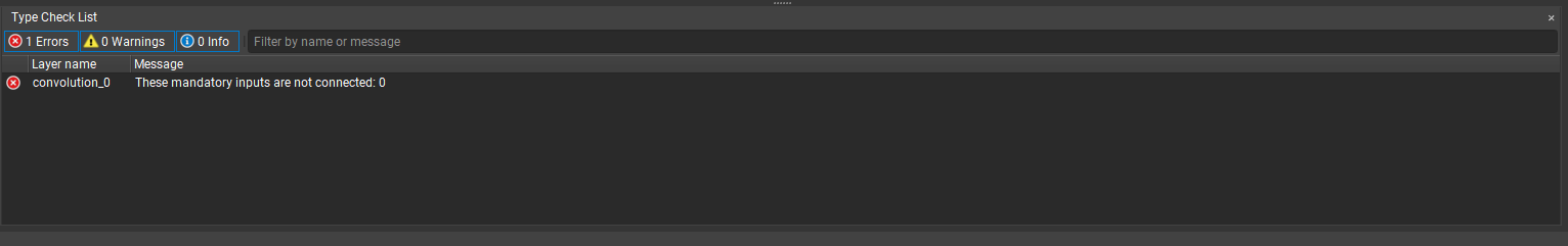
The most common layer error message you will see is These mandatory inputs are not connected. This merely indicates that the layer requires the indicated input terminal to be connected. Input terminal numbering is zero-based.
You can connect your own messages to the type checker when developing plugins. Log messages your plugins emit during parameter load and reshape (ILayer::loadFromParameters and ILayer::reshape) will be displayed automatically in the type checker.
2.5. Creating a Model
Dropping a layer into the canvas creates a new instance of that layer type with an automatically generated name. All instances must have a unique name that you can edit; names should be valid C++ identifiers. Layers are represented by a rectangular node on the canvas. This node shows the name, parameters, and activation function associated with the layer, as well as an icon if the type checker has reported any issues. When the mouse cursor is over a glyph, an icon appears at the bottom left of the glyph. Clicking it minimizes the layer to show only the icon and layer name. This can help to reduce the space taken by your network on screen. You can expand the glyph again using the same icon.
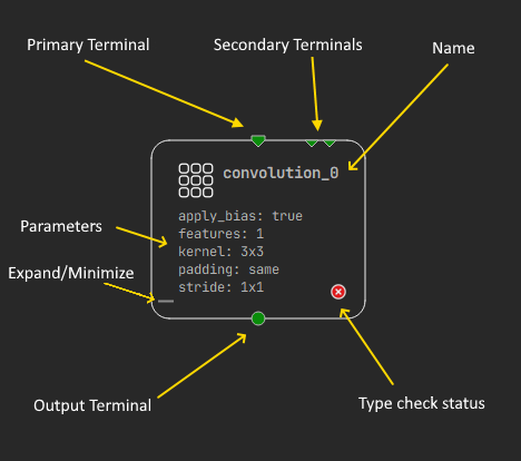
Layer glyphs represent the layer's inputs and outputs using terminals. Green triangles at the top of the node indicate inputs, and green circles at the bottom of the node indicate outputs. Most primary input terminals need to be connected for the network to be valid, but secondary input terminals are not mandatory. Secondary inputs that you do not provide directly in the network graph will typically be loaded from weights files during inference. Multiple links can start from the output terminal but only one link at a time can end in an input terminal.
Some layers use "infinite" inputs and accept an arbitrarily large number of inputs. Upon connection to an infinite terminal, more terminals are created on the glyph to allow for new connections.
See the layer's description in the editor's documentation browser (Help > Layer Documentation) for details of a specific layer's inputs and parameters.
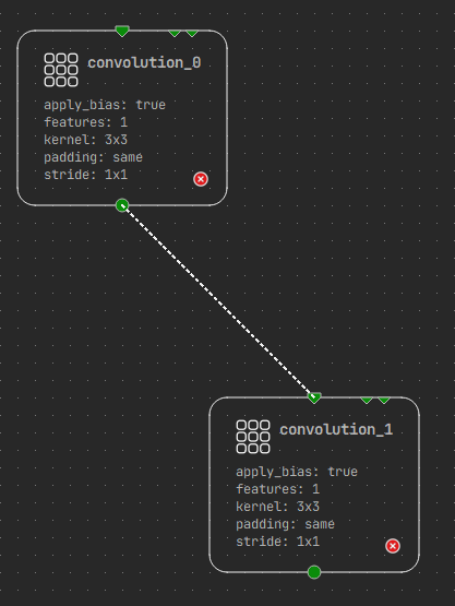
To connect a layer to another layer, click and hold from any terminal and drop to which terminal you wish to connect to. This action creates a link which segment can be moved for better visualization. Layers and links can be removed by selecting them and using the delete key.
Layers can be moved freely on the canvas by dragging them. This allows you to visually arrange your network and present an overview of your network. A background grid can be turned on with View > Show Grid to help align layers.
Enabling tensor shape display under View > Show Tensor Shapes, will show the tensor shapes information on links connected between two layers.
Double-clicking an unassigned input or output terminal on a layer node will create an input or output layer automatically and link it to that terminal.
2.6. Weights
Weights are used by both inference runs and during analysis. You can specify the folder which contains your model weight under the Tools > Network Settings dialog. NVIDIA Nsight Deep Learning Designer expects the weights folder to contain a weight file with Numpy format (see https://numpy.org/devdocs/reference/generated/numpy.lib.format.html) per layer and weight type following the naming convention: layerName_weightType.npy. Each weights' tensor should be stored in FP32/NCHW order. Standalone applications using NvNeural can provide their own weights loader.
2.7. Templates and Network Layers
It is common to find repetitive patterns in a neural network. To aid reusability and speed iterations, NVIDIA Nsight Deep Learning Designer supports the use of templates. A template is a self-contained group of layers connecting to the rest of the network.
To create a template, select the desired layers and use the Group command from the selection's context menu. The layers are reorganized into a template, and the new template is added to the palette. This template layer can then be added to any canvas and will act as if it is a single layer. Templates in the network can be ungrouped using the Ungroup context menu command. Ungrouping a template replaces it with the individual layers it represented.
Other networks from disk can also be imported as templates using the Edit > Import Model as Template command. Finally, you can export multiple template definitions on disk using the Edit > Export Template Definitions command; these templates definitions can be shared and loaded by others using the Edit > Import Template Definitions command. Any of these template importing methods will check against collision to avoid unwanted overwrite. In case of collision, NVIDIA Nsight Deep Learning Designer will ask you to choose between skipping the template import, renaming it, or overwriting the previous definition.
Parameters of layers contained in the template can be edited from the Settings dialog in the parameter editor for the template instance. You can then select which parameters to display and edit them in the parameter editor. Note that all the template instances share the same set of visible parameters.
Network layers are a special type of layer that represent a complete external network. Much like templates they act as a simple layer in the editor, but unlike templates, they can reference their own weights folder. Network layers are intended for workflows where users are sharing their networks and wish to integrate them as components of bigger networks.
External models can be imported using the Edit > Import Model as Layer command. Only local networks can currently be imported.
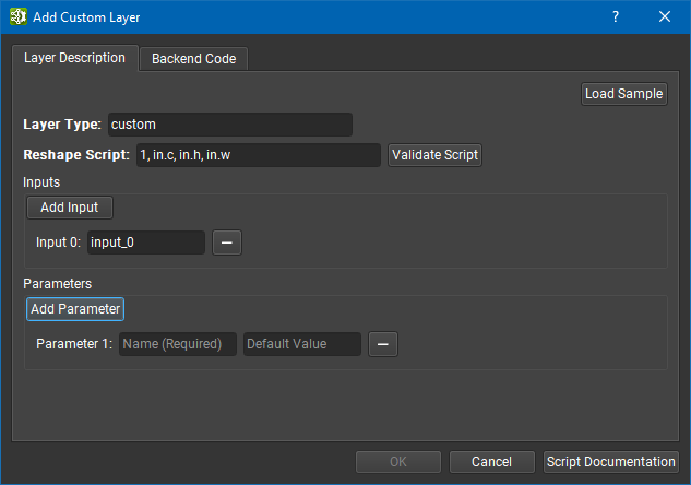
2.8. Custom Layers
Using custom layers, you can implement a new layer directly in the editor without having to use the NvNeural SDK. This method is faster but features are more restricted, so you should first assess if a custom layer can fit your need. To create a custom layer, use the dialog in Edit > Add Custom Layer. Custom layer creation is divided into two parts: the layer description and backend code. The layer description defines the layer type, inputs, and parameters. A scripting language is used to define the shape of the layer given its parameters and input sizes; refer to the Script documentation directly in the dialog box for details.
The following is an example of a reshape script for a space to depth layer:
in.n, in.c * 4, in.h / 2, in.w / 2
The in keyword represents the input tensor, and in.n, in.c, in.h and in.w are used to get the input tensor dimensions. Here, we are dividing by two the width and height while multiplying by four the channel count.
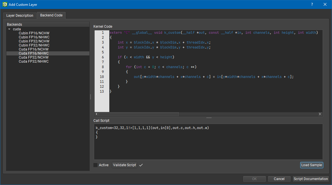
In the backend code sections, users define the implementation for each available backend and format for their layer. How the kernel is called is also specified using a scripting language.
Example of a kernel launch script:
k_custom<16,16,8!>[1,1,1,1](out,in[0],out.c,out.h,out.w){}k_custom is the name of the kernel to launch while <X, Y, Z> are the thread block dimensions, [1,1,1,1] can be used to specify stepping and finally you can pass arguments to the kernel. The kernel launch is sized to launch one CUDA thread per output element, increasing the number of blocks in the grid as necessary. If a particular block dimension is fixed for the kernel and does not need to be scaled as the input tensor size increases, add the ! suffix to that dimension component. In the <16,16,8! example above, the grid X and Y dimensions will be scaled as W and H increase, but the grid Z dimension is fixed at 1 and will not scale.
It is not mandatory to implement the layer for all variants of backend and format but at least one is necessary for the layer to be valid.
Once the custom layer is finished, just click OK in the dialog box. This will add the new custom layer to the list of available layers in the Layer palette.
2.9. Fusing Rules
One of the features of NVIDIA Nsight Deep Learning Designer and NvNeural is the ability to fuse layers or activations. This often results in a noticeable speed-up during execution with no significant decrease in quality. Fusing simply consists of executing a kernel performing the task of two or more correlated operations in a single pass, rather than a succession of single passes for each of these layers. Performing multiple operations in a single kernel reduces launch overhead and reduces memory traffic during evaluation, as key values are still present in registers or cache.
A fusing rule is a way to express the conditions under which we want a series of layers to be replaced by a specific layer. Typically the replacement layer is a fused layer, but the replacement layer can be an alternate implementation of the source layer or even an entirely different operation. Conditions can depend on the inputs of a layer or parameters of a layer as well as the current tensor format. In NVIDIA Nsight Deep Learning Designer, available fusing rules loaded from plugins can be viewed in the Fusing Rules tool window. Select a fusing rule to view its definition in the viewer at the bottom of the fusing rule window.
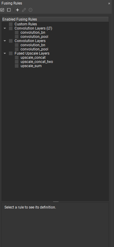
Individual fusing rules can be enabled or disabled using the checkboxes. You can define your own custom fusing rules directly in NVIDIA Nsight Deep Learning Designer, the fusing rule syntax is detailed in the Add Custom Rule dialog.
3. Inference
Inference can be performed on the current model using the Launch Inference quick action. Only one run can be launched at a time, but the launch is cancelable. Settings related to inference launch are located in the Network Settings dialog under the Tools menu. By default the network will be run using the FP16/NHWC tensor format for 10 iterations. If no weight folder or inputs are specified, the tool will generate random tensors. Using the Inference Run Logger tool window, you can get details of past and current inference runs. It is possible to copy the generated command line options passed to ConverenceNG if you wish to reuse it for a launch from a terminal. The average inference time for the whole network is also reported in the logger as well as in the generated report.
3.1. Profiling
Profiling can be turned on as part of the Network Settings for inference. If enabled, in-depth metrics at the network and layer levels will be collected during inference runs. The profiling results are available in the generated inference report.
3.2. Inference Report
An inference report is saved to disk after each inference run. The report is organized around the Layer Table, which contains the full list of layers and their details like name, type, output size, distance from input and average inference time. It is possible to switch between relative and absolute inference time using the corresponding button above the table.
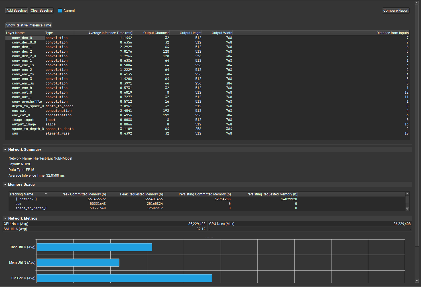
The Network Summary section contains the network average inference time as well as the tensor format used for the inference. If profiling was enabled for the associated run, then a Network Metrics section and a section per profiling metrics group is also present in the report. Each of them contains metrics values and charts. For layer level metrics, you must select the desired layer from the table to see the associated metrics values in the metrics sections.
Additionally, a Memory Usage section contains a table with memory usage tracking for each layer in the network. Note that persisting memory is allocated memory that was not freed before inference completed.
This table contains 4 columns:
-
Peak Committed Memory:
The maximum amount of memory a layer/the network held at any point during inference
-
Peak Requested Memory:
The maximum amount of memory a layer/the network requested at any point during inference
-
Persisting Committed Memory:
The amount of memory a layer/the network persisted during inference
-
Persisting Requested Memory:
The amount of memory a layer/the network requested to persist during inference
To compare multiple layers' metrics values together, use the baseline system accessible from the top of the report. By using the Add Baseline button, you can add the selected layer as a baseline. Each layer baseline is associated with a unique color that is used in charts to distinguish the layers. Use the Clear Baseline button to remove all the layer baselines.
3.3. Compare Inference Reports
When iterating on a model design, comparing inference reports can help pinpoint performance issues or validate proposed improvements. To compare reports either use the Compare Report button in an inference report or the Compare Inference Reports action under the Tools menu. In the dialog box you can compare multiple reports at once using the [+] button. The report comparison document is similar to the inference report. Each report being compared is assigned a unique color used in the comparison document to identify in charts.
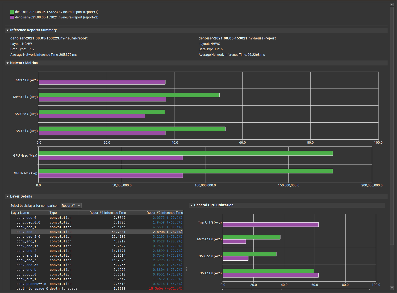
The Inference Reports Summary section groups the overview details of each report: tensor format and average inference time. If at least one of the reports contains profiling data, the Network Metrics section presents a chart with the network level metrics. Finally, the Layer Details section is composed of two elements: the layer table and the collected metric charts.
The Layer Table contains the layers from all the reports, layers that share the same name and layer type across reports are compared across reports. The comparison document shows the difference of average inference time of layers across reports. The report to use as the basis for that comparison can be selected using the combo box above the layer table. Select any layer from the table to see the metrics value of that layer across reports with profiling data.
4. Analysis
Inference reports permit us to assess the performance and find bottlenecks of a model, but on the other hand, the Analysis Mode makes it easier to verify the quality of the model and review the individual channels of layer tensors.
Analysis layers are layers that are designed primarily to work with the analysis system rather than in production networks. They provide interactive controls for tweaking the model. The most commonly used analysis layer is the mix layer: given two inputs, it blends them with a configurable mix factor and blend function. This is useful to compare the result of a Denoiser network with the initial input image. If a model contains a mix layer, it is possible during analysis to modify the parameters of the mix layer interactively and see the live impact on the model’s output. Other analysis layers support affine transforms, noise injection, and other visualizations. Look in the Analysis category of the layer palette to see the provided operations.
For meaningful results during analysis, it is necessary to provide a weights folder for the model. The weights folder settings can be found under the Network Settings dialog in the Tools menu. In order to switch to analysis mode, click on the Launch Analysis action from the quick action menu. During analysis mode, all opened models are set to read-only mode; they cannot be edited while analysis is running. To switch back to editing mode, click on the Stop Analysis button from the quick action menu.
4.2. Model Inputs
The model input tool window is used to select files to load for each input layer in the model. Supported file types are: images (PNG, JPG), videos (AVI, MPEG, MKV, WMV), and NumPy tensors (NPY).
To load a file for a given input, double-click on the input viewer or right-click and Open Input File. If the file is a video file, you can use the video controls under each input viewer to either play, pause, or set the video to a specific spot. Numpy files are transformed into images for visualization purposes, but are passed as-is to the actual network.
4.3. Parameter Editor
Layers from the model that provide runtime-modifiable options can be edited during analysis in the Parameter Editor tool window. Layers may contain multiple options (as defined by the IRuntimeOptionsLayer interface in NvNeural), and are grouped under an expandable item. Updating the value of a runtime option reruns the network to show the effects of your change.
All layers inside the Analysis Layers plugin implement runtime options. Refer to the specific layer documentation pages in the editor for more details.
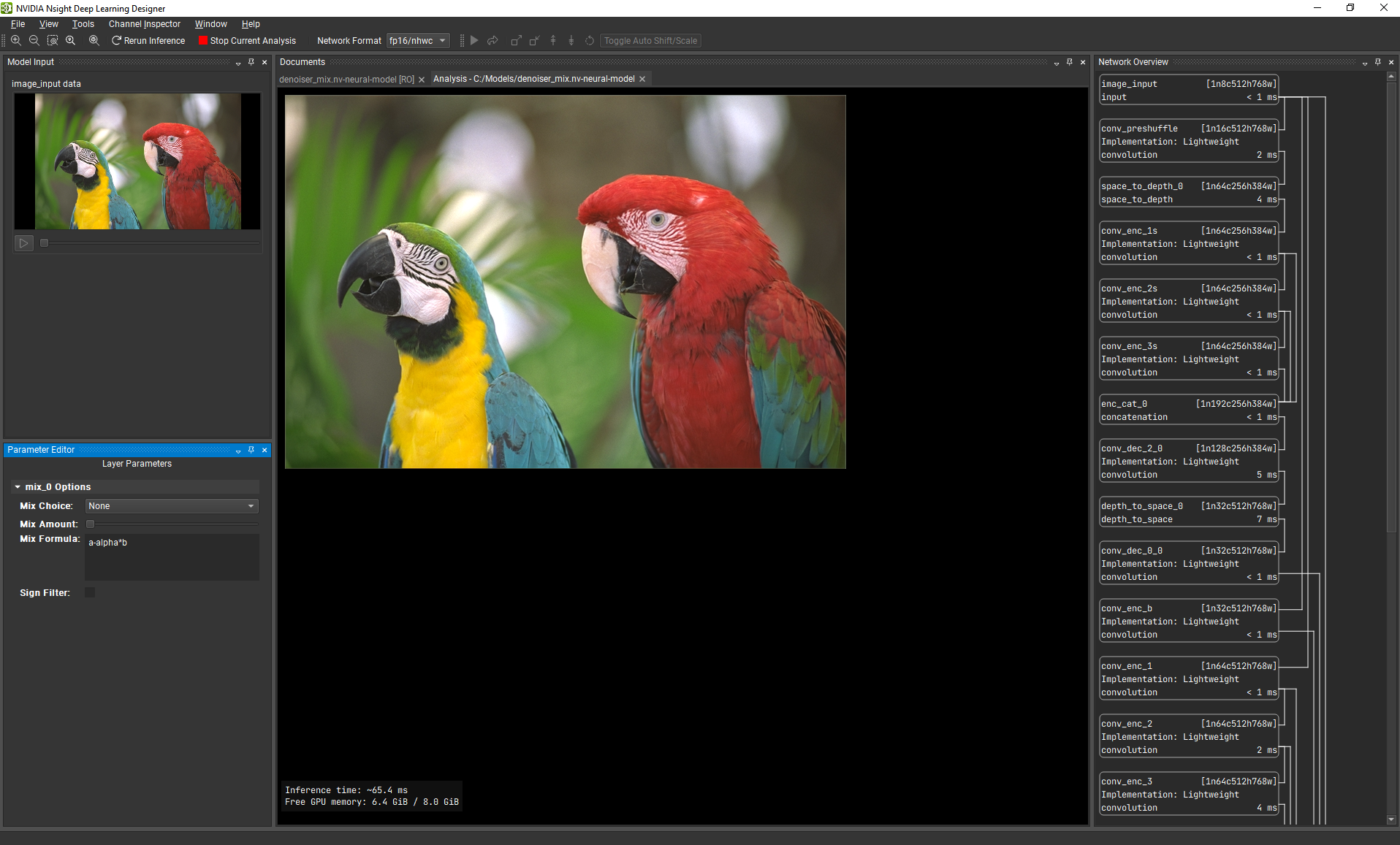
4.4. Network Overview
The Network Overview shows a flattened version of the model graph; its order reflects the internal execution order of the model. Each layer glyph contains the name, type, and current shape of the layer; some layers might also show status messages. Layer connections are represented in the graph using links. Select any layer highlights its input links in yellow and output links in blue.
If profiling timing is enabled, controllable with Tools > Profile Layer Timings, each layer will display its most recent inference time. It is necessary to rerun inference when enabling layer timings in order to collect timing data; do this using the Rerun inference button from the quick action menu.
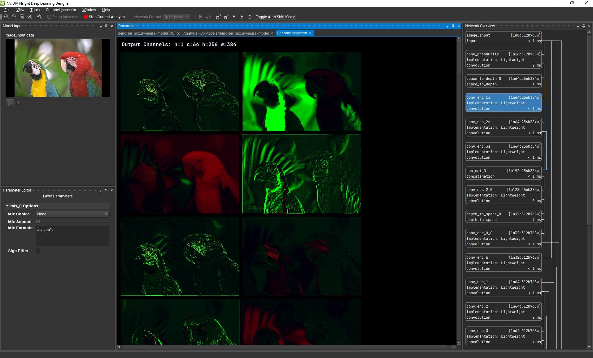
4.5. Channel Inspector
The Channel Inspector can be used to analyze a layer's channels and weights, and can debug into the network. To open the Channel Inspector, use the View > Channel Inspector menu item or toolbar button. You can also double-click on a layer in the Network Overview. Switch between the Analysis Output view and the Channel Inspector by clicking on their respective tabs. The Channel Inspector tab can be closed and reopened during analysis, but closing the Analysis Output view will stop analysis and close the Channel Inspector.
4.5.1. Layer's Channels
To view a layer’s channels you need to select the layer from the Network Overview. Channels and weights are presented as N * C slices of size H * W. We transform feature maps into images using a red/green colormap.
It is possible to adjust the shift and scale of the transformation using either the quick actions or the shift and scale actions from the Channel Inspector menu. The Reset Parameters action reset the shift and scale values.
Note that for large feature maps, the visualizer can take some time to load. The feature maps displayed are always from the latest inference pass, for networks using video feed features maps will be updated alongside the video feed
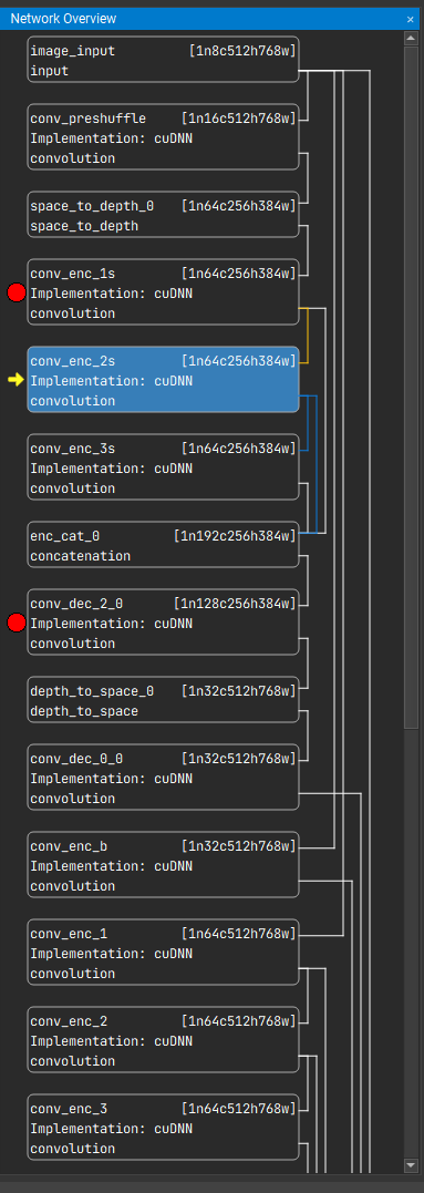
4.5.2. Debugger
It is possible to set breakpoints at a layer level. To do so, right-click on a layer from the Network Overview and select Add Breakpoint. If the network is not currently being debugged, this will set a new breakpoint and also stop the current network execution at that layer. Similarly, you can remove breakpoints by selecting any layer with a breakpoint, right-clicking on it and selecting Remove Breakpoint.
During debugging, it is possible to visualize other layers, feature maps, step to the next layer, or resume the current execution. If you resume the execution while there are no more breakpoints in the network, then it will quit the debugging mode.
Video feeds are synchronized with the debugging state; the feed is paused when the network execution is paused, and new frames are requested from the video source only when network execution touches the associated input layer. To resume normal video playback, exit the debugger by removing all breakpoints and resuming network execution.
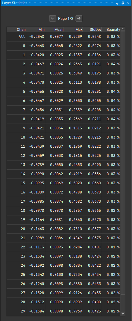
4.5.3. Layer Statistics
The Layer Statistics window shows statistics value for each channel of a
layer while in the channel inspector. After selecting a layer from the Network Overview window, a table with the corresponding
statistical values will be displayed. The table only shows at most 32 channels; if the
selected layer has more than 32 channels, you can use the next and previous page button
to access the other channel values. The first row contains the statistical value for the
layer as a whole.
The table contains 6 columns: the channel index, mininum, mean,
maximum, standard deviation and sparsity. The sparsity is given as a percentage
representing how many values in the channel are close to 0.
5. Exporters
NVIDIA Nsight Deep Learning Designer offers multiple ways to deploy your model to an application.
The following table shows the current support of NvNeural layers for the ONNX, DirectML and PyTorch exporters:
Layer
DirectML
ONNX
PyTorch
affine
no
yes
yes
batch_normalization
yes
yes
yes
color_conversion
no
no
no
concatenation
yes
yes
yes
convolution
yes (partial)
yes
yes
conv_bn
no
no
no
conv_pool
no
no
no
depth_to_space
yes
yes
yes
dropout
yes (removed)
yes
yes
element_wise
yes
yes
yes
fully_connected
no
yes
yes
gram_matrix
no
no
yes
instance_normalization
yes
yes
no
linear_blend
no
no
yes (partial)
lrn
yes
yes
no
mix
no
no
no
mono_four_stack
no
no
no
mono_to_rgb
no
no
no
noise
no
no
no
padding
yes
yes (partial)
yes
pooling
yes
yes
yes
resize
no
no
no
selector
no
no
no
slice
yes
yes
yes
snapshot
no
no
no
space_to_depth
yes
yes
yes
upsample
yes
yes
yes
upscale_concat
no
no
no
upscale_concat_two
no
no
no
upscale_sum
no
no
no
zero_embed
no
no
yes
Specific notes:
-
Dropout layers are removed from the DirectML inference graph during export.
-
The apply_bias parameter for convolutions is not supported at this time by the DirectML exporter.
-
The mono_four_stack and mono_to_rgb layers are provided as samples of custom HLSL-based operators, and are not innately supported by DirectML.
-
The replication mode of padding layers is not supported by the ONNX exporter.
The following table lists the current support of NvNeural activations for the ONNX, DirectML, and PyTorch exporters:
Activation
DirectML
ONNX
PyTorch
leaky_relu
yes
yes
yes
leaky_sigmoid
no
no
no
leaky_tanh
no
no
no
relu
yes
yes
yes
sigmoid
yes
yes
yes
softmax
yes
yes
yes
sine
yes (not fusable)
yes
no
tanh
yes
yes
yes
Specific notes:
-
Sine activations are implemented in DirectML as DML_OPERATOR_ELEMENT_WISE_SIN operators, which are not supported as fusable activations inside DML_OPERATOR_DESC structures. They are instead broken out into separate DirectML operators with in-place execution.
5.1. Generating ONNX
To export your model to ONNX, click on the ONNX Model action under the File > Export sub-menu. This will generate an ONNX model following your model design and parameters. Note that the ONNX support is not exhaustive and some layers, activations, or parameter combinations might not export correctly. Most unsupported layers can be replaced by custom operator placeholders. You are encouraged to check the exported network using an ONNX graph visualizer or type-checking tool to ensure correctness before trying to run the network.
Some behaviors of the ONNX exporter can be controlled in the Settings dialog.
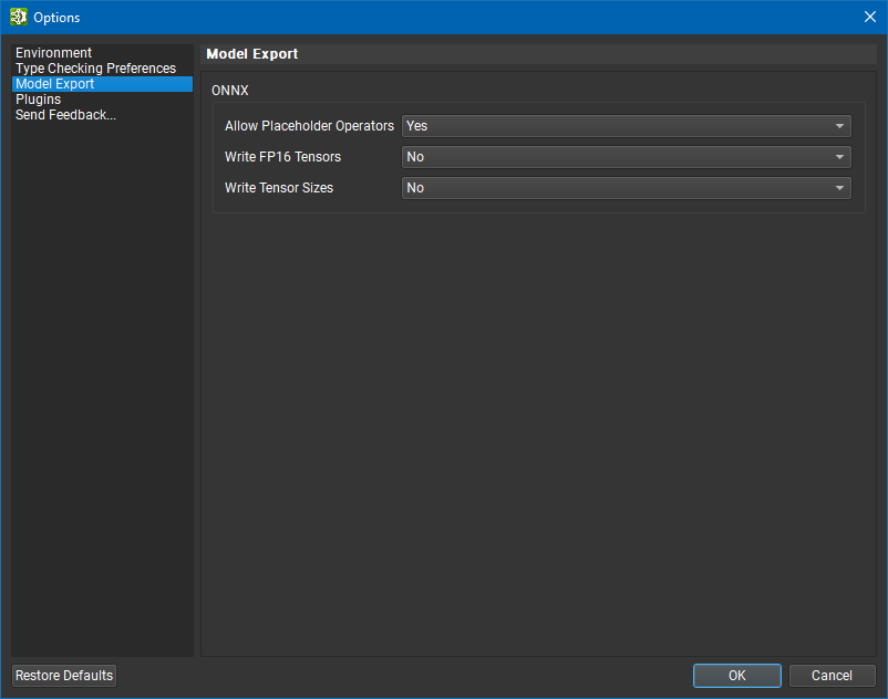
The following options are currently available:
-
Allow Placeholder Operators – When this option is set to Yes, the exporter creates placeholder nodes for activations and layers that are not supported by the ONNX standard operator set. These nodes use the com.nvidia.nvneural.placeholders operator set namespace. Layer parameters that cannot be represented using the default onnx.ai operator set will still generate warnings or errors during export.
When this option is set to No, the exporter will fail instead of generating placeholders.
-
Write FP16 Tensors – When this option is set to Yes, the exporter will convert graph inputs, outputs, and weights initializers to FLOAT16 tensors instead of FLOAT. Some ONNX inference frameworks rely on the presence of FLOAT16 tensors to enable fp16 inference modes.
When this option is set to No, the exporter will emit FLOAT types for inputs, outputs, and weights initializers.
-
Write Tensor Sizes – The current versions of the ONNX format specification and ONNX Runtime framework allow tensor sizes (such as for graph inputs and outputs) to be specified using “dimension variables” that are resolved at runtime. This feature allows for resolution-independent inference similar to NvNeural, but not all ONNX tools support it. When this option is set to Yes, the exporter emits explicit tensor sizes based on the sizes reported by NvNeural for increased compatibility.
When this option is set to No, the exporter emits tensor sizes using dimension variables.
5.2. Generating a C++ Project with NvNeural
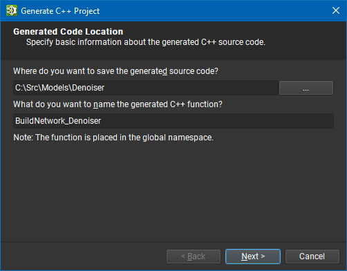
If you want to export the model you designed inside NVIDIA Nsight Deep Learning Designer to an executable application, you can use the Generate C++ Project action under the File > Export sub-menu. This will export your model to a C++ project that relies on our inference framework: NvNeural. Performances of the application is more likely to match what you can profile in NVIDIA Nsight Deep Learning Designer, since they both use the NvNeural framework.
The wizard guides you through the exporting process. First, you must specify the target folder to export the project to, and the name of the main network builder function.
The second page lets you choose if you want the exporter to generate additional code for a sample CLI application. The CLI allows you to choose the input files, output files, tensor format, number of iterations, and weights folder when running the network. The second option adds a CMake project file to build the generated project using the CMake system.
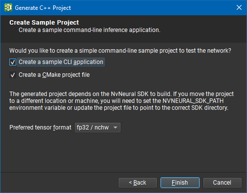
After selecting the preferred network tensor format, click on Finish. A dialog box will report if generation was successful or list any errors. Its Details pane additionally shows the command line used to launch the exporter.
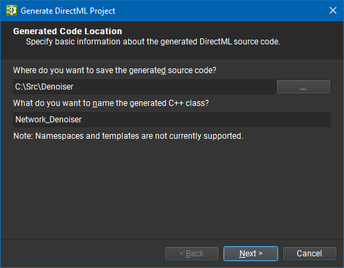
5.3. Generating a C++ Project with DirectML
If you wish to generate an application from your model that uses DirectML as the inference framework, click on Generate DirectML Project under the File > Export sub-menu. This feature requires the Windows version of Nsight Deep Learning Designer. The application uses our intermediate API NvDml that takes care of the lower-level calls to the DirectML and Direct3D 12 APIs. Sample client application code in the generated Main.cpp provides simple input/output support and weights loading; in more complex applications you can replace these routines with direct management of ID3D12Resource buffers.
The wizard guides you through the exporting process. First, you must specify the target folder to export the project to, and the name of the generated class that will contain the network construction logic.
The second page lets you choose if you want the exporter to generate additional code for a sample CLI application. The CLI allows you to choose the input files, output files, tensor format, number of iterations and weights folder when running the network. The second option adds a CMake project file to build the generated project using the CMake system.
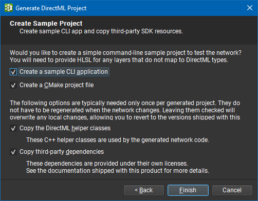
Click the Finish button to export. A dialog box will report if generation was successful or list any errors. The Details pane additionally shows the command line used to launch the exporter.
The DirectML project generator emits hooks for custom operator HLSL when no suitable DML feature level 3.0 operator exists. See the nvdml::CustomOperatorBase class for details of this interface. As with NvNeural, the weights loading and input systems are fully replaceable; we recommend integrating your own resource management systems in production applications rather than relying on the teaching-focused sample code.
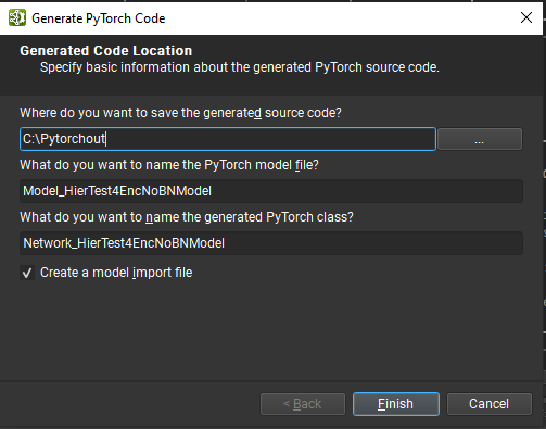
5.4. Generating PyTorch code
NVIDIA Nsight Deep Learning Designer does not target the training phase of designing a Deep Learning network, but as it is an indivisible part of the workflow it is possible to export models created in NVIDIA Nsight Deep Learning Designer to a PyTorch model.
PyTorch export support is currently experimental, not exhaustive, and some models might not export correctly. We will add further support for exporting to training frameworks in future releases.
To use the PyTorch exporter, click on the Generate PyTorch files command under the File > Export submenu. The wizard guides you through the exporting process. You must specify the target folder to export the project to, and the name of the main network builder function. Optionally, you can choose to have all the necessary module imports separated in a single importable Python module.
The exporter requires that you have a suitable configured Python environment with at least the following packages installed:
6. Main Menu and Toolbar
Information on the main menu and toolbar.
6.1. Editing Mode

6.1.2. Main Toolbar
The main toolbar shows commonly used operations from the main menu. See Main Menu for their description.
In addition, the toolbar contains the following commands:
6.2. Analysis Mode

6.2.2. Main Toolbar
The main toolbar shows commonly used operations from the main menu. See Main Menu for their description. In addition, the toolbar contains the following commands:
-
Rerun Inference
Rerun inference.
-
Stop Current Analysis
Stop the current analysis and swtich back to editing mode.
-
Network Format
Change the network format used for analysis.
Notices
Notice
ALL NVIDIA DESIGN SPECIFICATIONS, REFERENCE BOARDS, FILES, DRAWINGS, DIAGNOSTICS, LISTS, AND OTHER DOCUMENTS (TOGETHER AND SEPARATELY, "MATERIALS") ARE BEING PROVIDED "AS IS." NVIDIA MAKES NO WARRANTIES, EXPRESSED, IMPLIED, STATUTORY, OR OTHERWISE WITH RESPECT TO THE MATERIALS, AND EXPRESSLY DISCLAIMS ALL IMPLIED WARRANTIES OF NONINFRINGEMENT, MERCHANTABILITY, AND FITNESS FOR A PARTICULAR PURPOSE.
Information furnished is believed to be accurate and reliable. However, NVIDIA Corporation assumes no responsibility for the consequences of use of such information or for any infringement of patents or other rights of third parties that may result from its use. No license is granted by implication of otherwise under any patent rights of NVIDIA Corporation. Specifications mentioned in this publication are subject to change without notice. This publication supersedes and replaces all other information previously supplied. NVIDIA Corporation products are not authorized as critical components in life support devices or systems without express written approval of NVIDIA Corporation.