Inverse FFT

Overview

Inverse FFT implements the inverse Fourier Transform for 2D images, supporting real- and complex-valued outputs. Given a 2D spectrum (frequency domain), it returns the image representation on the spatial domain. It is the exact inverse of FFT algorithm.

Input as a magnitude spectrum	Output in spatial domain

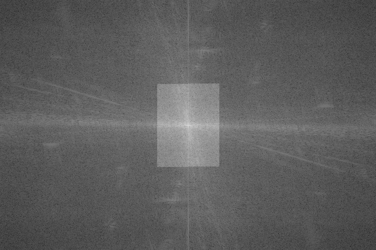Implementation

The inverse Fast Fourier Transform follows closely forward FFT's implementation, except for the sign of the exponent, which is positive here.

\[ I[m,n] = \frac{1}{MN} \sum^{M-1}_{u=0} \sum^{N-1}_{v=0} I'[u,v] e^{+2\pi i (\frac{um}{M}+\frac{vn}{N})} \]

Where:

• \(I'\) is the input image in frequency domain
• \(I\) is its spatial domain representation
• \(M\times N\) is input's dimensions

The normalization factor \(\frac{1}{MN}\) is applied by default to make IFFT an exact inverse of FFT. As this incurs in a performance hit and normalization might not be needed, user can pass the flag VPI_IFFT_DENORMALIZED to vpiSubmitIFFT to indicate that output must be left denormalized.

As with direct FFT, depending on \(N\), different techniques are employed for best performance:

• CPU backend
  • Fast paths when \(N\) can be factored into \(2^a \times 3^b \times 5^c\)
• CUDA backend
  • Fast paths when \(N\) can be factored into \(2^a \times 3^b \times 5^c \times 7^d\)

In general the smaller the prime factor is, the better the performance, i.e., powers of two are fastest.

IFFT supports the following transform types:

• complex-to-complex, C2C
• complex-to-real, C2R.

Data Layout

Data layout depends strictly on the transform type. In case of general C2C transform, both input and output data shall be of type VPI_IMAGE_FORMAT_2F32 and have the same size. In C2R mode, each input image row \((X_1,X_2,\dots,X_{\lfloor\frac{N}{2}\rfloor+1})\) of type VPI_IMAGE_FORMAT_2F32 containing only non-redundant values results in row \((x_1,x_2,\dots,x_N)\) with type VPI_IMAGE_FORMAT_F32 representing the whole image. In both cases, input and output image heights are the same.

Usage

1. Initialization phase
   1. Include the header that defines the inverse FFT functions.

      #include <vpi/algo/FFT.h>

   2. Define the input spectrum image. Since we're performing a C2R IFFT, the input width must be \(\lfloor \frac{w}{2} \rfloor+1\), where \(w\) is the output image width. Input and output heights must match. Image format must be VPI_IMAGE_FORMAT_2F32.

          VPIImage input = /*...*/;

   3. Create the output image. Again, because of C2F IFFT, the output type must be VPI_IMAGE_FORMAT_F32. We're passing 0 as flags to make the function return a normalized output.

          VPIImage output;
          vpiImageCreate(w, h, VPI_IMAGE_FORMAT_F32, 0, &output);

   4. Create the IFFT payload on the CUDA backend. Input is complex and output is real. Problem size refers to output size.

          VPIPayload ifft;
          vpiCreateIFFT(VPI_BACKEND_CUDA, w, h, VPI_IMAGE_FORMAT_2F32, VPI_IMAGE_FORMAT_F32, &ifft);

   5. Create the stream where the algorithm will be submitted for execution.

          VPIStream stream;
          vpiStreamCreate(0, &stream);

2. Processing phase
   1. Submit the IFFT algorithm to the stream, passing the input spectrum and the output buffer. It'll be executed on the CUDA backend, since the payload is created there.

          vpiSubmitIFFT(stream, ifft, input, output, 0);

   2. Wait until the processing is done.

          vpiStreamSync(stream);

   3. Now display output using your preferred method.
3. Cleanup phase
   1. Free resources held by the stream, the payload and the input and output images.

          vpiStreamDestroy(stream);
          vpiPayloadDestroy(ifft);
          vpiImageDestroy(input);
          vpiImageDestroy(output);

For more details, consult the API reference.

Limitations and Constraints

Constraints for specific backends supersede the ones specified for all backends.

All Backends

• The following input image types are accepted:
  • VPI_IMAGE_FORMAT_2F32 - complex input.
• The following output image types are accepted:
  • VPI_IMAGE_FORMAT_F32 - real output.
  • VPI_IMAGE_FORMAT_2F32 - complex output.

CPU

• If output has type VPI_IMAGE_FORMAT_F32, its width must be even.
• Input and output rows must be aligned to 4 bytes.

CUDA

• There can be memory allocation in first call to vpiSubmitIFFT and every time the input or output row stride changes with respect to previous call.

PVA and VIC

• Not implemented.

Performance

For information on how to use the performance table below, see Algorithm Performance Tables.
Before comparing measurements, consult Comparing Algorithm Elapsed Times.
For further information on how performance was benchmarked, see Performance Measurement.

clear filters Device: Jetson AGX Xavier Jetson TX2 Jetson Nano  -  Streams: 1 4 8