

Error Analysis
The accuracy of a particle-mesh calculation depends on how well the splitting represents the physical interaction and how accurately the mesh evaluates it. Intrinsic error belongs to the decomposition itself. Extrinsic error arises from discretization onto a mesh, including its finite Fourier range, spreading, aliasing, and interpolation.
The convergence plots compare energies and forces at fixed particle positions. The NVE study tests a different property: how well the resulting dynamics conserve energy over time.
Intrinsic and extrinsic error
We follow the definition in Section IV A of Predescu et al., The u-series: A separable decomposition for electrostatics computation with improved accuracy, The Journal of Chemical Physics 152, 084113 (2020):
We start by focusing on errors that are intrinsic to the decomposition scheme: those that remain even if the direct and k-space sums are performed exactly.
Fix the decomposition parameters, including its prescribed short-range cutoff, and evaluate its direct and complete Fourier sums exactly, with matching self and boundary corrections. Any remaining difference from the physical interaction is intrinsic. Here, extrinsic names the additional error from evaluating that decomposition on a mesh.
Intrinsic error: the decomposition itself
A decomposition can define an approximate pair interaction even before a mesh is introduced. For example, cutting off or shifting the Ewald short-range kernel changes the interaction it represents. The u-series is exact within its prescribed cutoff but approximates beyond it. These discrepancies remain when the sums for the chosen decomposition are evaluated exactly.
An exact decomposition has no intrinsic error under this definition. In the C2 Prolate construction, beyond , and is its exact complement inside the cutoff. Those mathematical functions therefore reconstruct everywhere. This statement concerns the decomposition; its evaluation on a finite mesh still has error.
In particular, its Fourier kernel has a nonzero tail. Omitting modes to fit a finite mesh introduces extrinsic error. Evaluating every retained coefficient exactly does not recover the omitted modes.
Extrinsic error: discretization onto a mesh
The ideal reciprocal sum uses the point-charge structure factor
The mesh method approximates this calculation through spreading, an FFT, Fourier scaling, and gathering over a finite set of modes. Its error depends on the grid spacing, assignment window and support, deconvolution rule, and how forces are recovered at particle positions. Sampling introduces aliases; interpolation introduces further approximation. Deconvolution compensates the assignment window, but cannot recover omitted modes or remove all aliasing. The spreading guide derives those steps.
The same window can give different errors with different splittings because each physical Fourier kernel weights the affected modes differently.
How to separate the contributions
Let be the force from the physical interaction, the force from exact evaluation of the chosen decomposition, and the force after mesh discretization. Use exact kernels and arithmetic at the same particle positions and box, with consistent boundary and correction conventions:
Their vector sum is , the force error of the mesh approximation under these assumptions. The same subtraction separates signed energy errors. Error magnitudes generally do not add: the contributions can reinforce or cancel one another.
To measure them separately, first converge the evaluation of the chosen decomposition and compare it with a converged physical reference. Then compare the practical mesh result with that decomposition result. In practical calculations, polynomial kernel fits, tabulated Fourier coefficients, and floating-point roundoff can affect both evaluations. Control these effects when measuring either contribution.
The plots below use finite precision and a reference with finite resolution. They include intrinsic and extrinsic errors together with the effects of kernel evaluation, roundoff, and the reference itself.
Mesh convergence
The plots below vary the number of grid points while keeping the splitting parameters and real-space cutoff fixed. They show energy and force errors at 6 Å and 9 Å cutoffs. Increasing the grid size expands the retained Fourier range and changes the assignment error. The decomposition stays fixed, so its intrinsic error is unchanged while these extrinsic contributions vary.
All curves use the same C2-order-3 (C2O3) spreading and interpolation window with discrete deconvolution. C2O3 names the assignment window; C2 Prolate names the splitting. Holding the window fixed allows the splittings to be compared with the same assignment rule, though mesh error remains. The Ewald curves therefore use this common mesh calculation rather than stock OpenMM PME. The cuPotential curves are shown in green.
What the axes measure
The horizontal axis is , the number of mesh points per axis. Each calculation uses a mesh; for a cubic box of side , its spacing is . The study samples .
Each saved frame is compared with an OpenMM double-precision reference. The upper panels show the relative energy error of the interaction channel:
The lower panels show the relative force error across all particles:
Here, “total” includes the direct and reciprocal contributions and their self and exclusion corrections within one interaction channel. Coulomb and attractive dispersion are evaluated separately. The force metric measures the norm of the error over all particles; it is not the largest per-particle error or the error in the complete molecular force field.
Frame averages and error bars
Each point combines saved NPT frames. For either error metric, the mean and standard deviation of the logarithmic errors are
The plotted value is the geometric mean , and the error-bar endpoints are and . These bars describe variation between the saved frames; they are not confidence intervals. The dashed line in the force panels is a comparison guide, not a bound that every frame must satisfy.
Coulomb convergence
The Coulomb channel uses the physical interaction. The comparison includes Ewald splitting, u-series 2, and cuPotential’s C2 Prolate splitting. Within each cutoff panel, their splitting parameters stay fixed while the mesh changes.
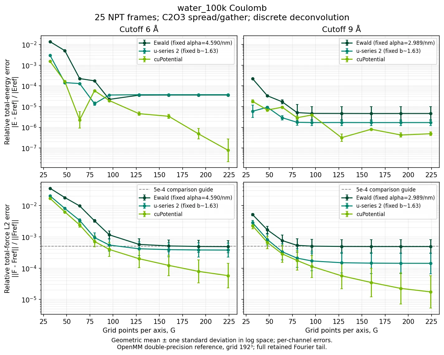
Coulomb convergence for the saved water system. Columns show the 6 Å and 9 Å cutoffs; rows show energy and force errors. All curves use C2O3 spread/gather and discrete deconvolution. The reference uses OpenMM PME in double precision with a mesh.
The cuPotential force error falls across most of the sweep. The fixed Ewald and u-series curves level off sooner. These are total-error curves: they show where refinement stops helping for these settings, but do not isolate the intrinsic or extrinsic contribution. Energy errors need not decrease monotonically: contributions can cancel without a corresponding reduction in force error.
Attractive dispersion convergence
The dispersion channel is the attractive interaction. Its reference uses OpenMM LJPME with the repulsive contribution subtracted. Consequently, these plots describe attractive dispersion rather than the full Lennard-Jones potential.
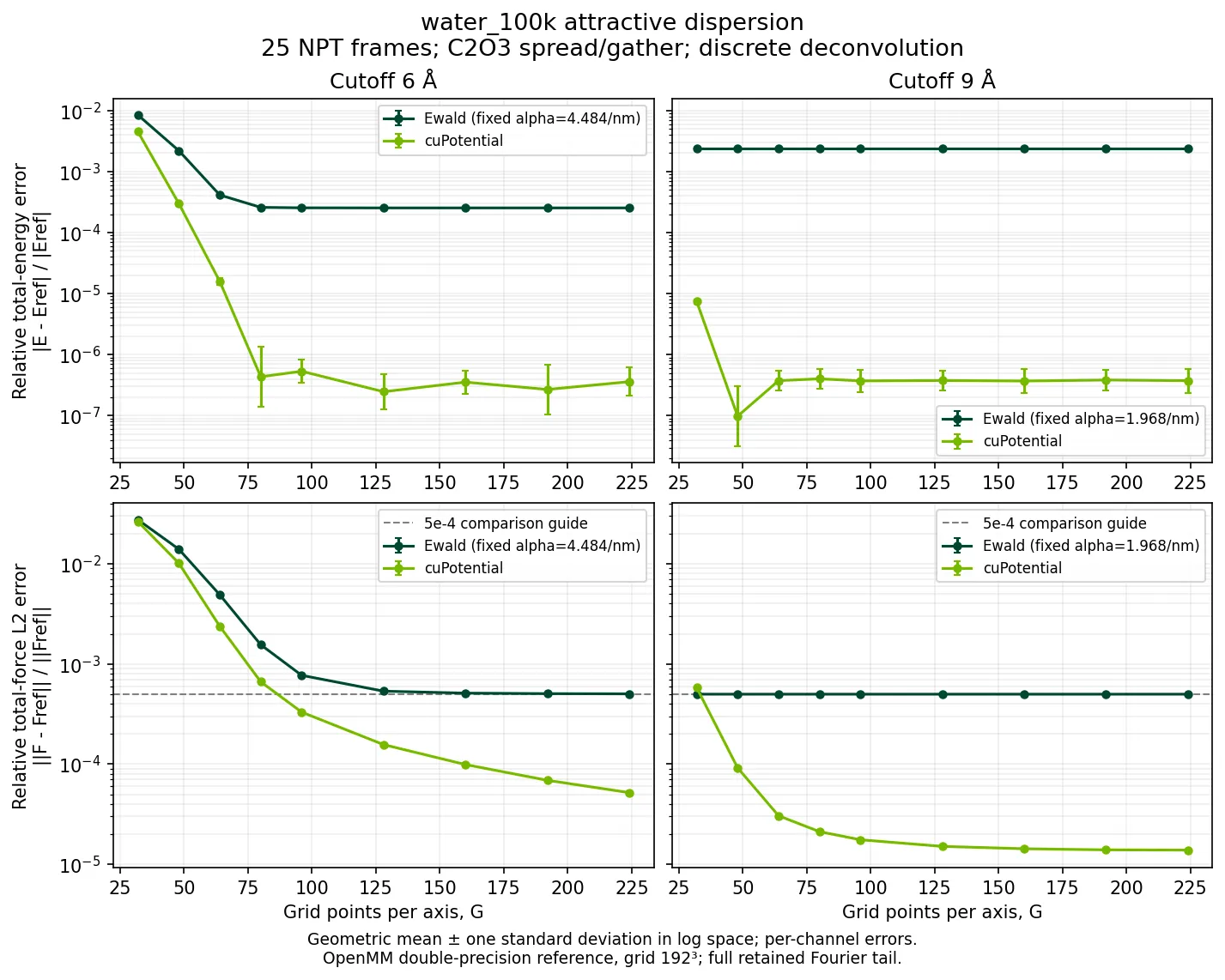
Attractive dispersion convergence for the same saved frames. The splitting parameters, C2O3 spread/gather, and discrete deconvolution are fixed within each panel. The reference uses OpenMM LJPME in double precision with a mesh, after removing the repulsive contribution.
At 6 Å, the cuPotential force error decreases throughout the tested range. At 9 Å, it begins to level off on the finer meshes. The fixed Ewald curves plateau earlier. As in the Coulomb comparison, the plateau is an observation about the complete calculation, not a measurement of the splitting error alone.
Why a curve can level off
A plateau means that increasing alone is no longer reducing the dominant observed error. Several mechanisms can produce it:
The C2 Prolate curves retain every mode available on each mesh. A plateau does not establish an intrinsic error floor. To identify its cause, converge the Fourier sum for the chosen decomposition, vary the assignment window or its support, and check kernel evaluation and reference accuracy.
The splitting parameters were not retuned during these sweeps. The results describe these parameter choices and this water system; they are not separate measurements of intrinsic splitting accuracy or comparisons at equal cost.
Study conditions and reference resolution
The reference was also checked on the first frame using a mesh. The relative differences between the and reference calculations were:
These checks show the change in the reference on the first frame. They do not bound its error over all 25 frames. Near this scale, a difference from the reference cannot be attributed entirely to either intrinsic or extrinsic error in the method being tested.
NVE energy drift
We run these trajectories in the microcanonical (NVE) ensemble. Many factors can affect energy drift; here we focus on the contribution from any residual jump at the cutoff of the short-range splitting term. Tight constraint tolerances and Lennard-Jones switching help reduce other sources of drift.
This saved study compares cuPotential, standard OpenMM PME, and a converged PME reference over 10 ns for 10,000 rigid TIP3P-FB water molecules (30,000 atoms). All three trajectories start from the same positions and velocities and use a 2 fs timestep.
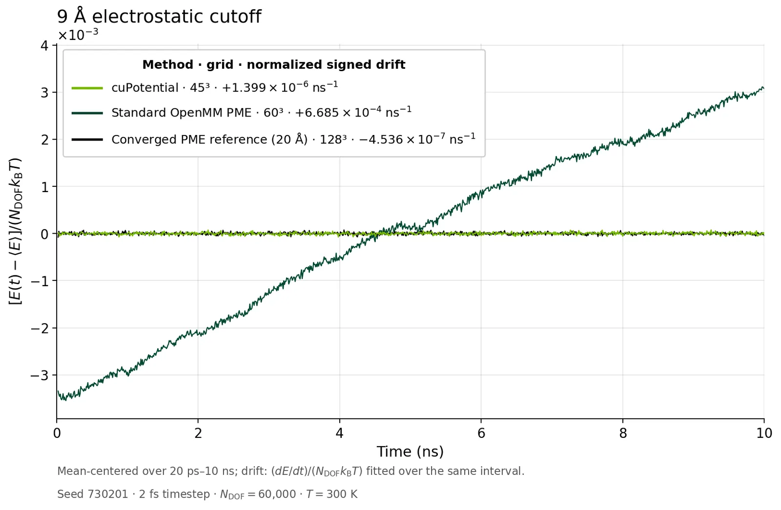
The cuPotential and standard PME runs use a 9 Å electrostatic cutoff. The reference uses a 20 Å cutoff. Each trace is centered on its own mean energy over 20 ps–10 ns.
Normalization and fitted drift
The vertical axis is
The study uses : three coordinates per atom, minus the rigid-water constraints. The normalization uses a fixed reference temperature . Centering removes each trajectory’s energy offset; it does not change its drift.
The legend reports the signed slope of a linear least-squares fit, normalized by the same energy scale:
The fit uses all 49,901 energy samples, recorded every 0.2 ps from 20 ps to 10 ns. The plotted curves show every 10 ps. A positive slope means energy increases; a negative slope means it decreases.
At these settings, standard PME has a clear positive drift, while cuPotential and the reference show much smaller drift on the same scale. This difference cannot be assigned to the splitting alone: the methods also use different meshes and reciprocal-space evaluation rules.
Simulation conditions
- Initial state: the same water configuration and velocities, with seed 730201, in a fixed cubic box of side 6.698671 nm.
- Integration: synchronized velocity-Verlet with RATTLE constraints, a 2 fs timestep, and constraint tolerance . Production uses no thermostat, barostat, or center-of-mass velocity removal.
- Precision: OpenMM 8.4 on CUDA, with mixed precision for all three methods.
- Electrostatics: standard PME uses automatic parameter selection at error tolerance ; the reference fixes and a grid.
- Lennard-Jones interactions: all three methods use the same 9 Å cutoff, a switching function starting at 8 Å, and no dispersion tail correction.
Future directions
Future work will likely re-optimize the numerical parameters to minimize ensemble error, rather than focusing primarily on force errors at fixed configurations.