Best Practices for Building and Deploying Recommender Systems
Abstract
This document describes the best practices for building and deploying large-scale recommender systems using NVIDIA GPUs. These practices are the culmination of years of research and development in GPU-accelerated tools for recommender systems, as well as building recommender systems for our in-house products and top-performing solutions for international recommendation systems competitions.
Recommender systems are the economic engine of the Internet. These applications have a direct impact on our daily digital lives in which they filter products and services among an overwhelming number of options, easing the paradox of choice that most users face.
The primary goal of this document is to provide best practices for building and deploying large-scale recommender systems using NVIDIA® GPUs. These best practices are the culmination of years of research and development in GPU-accelerated tools for recommender systems, as well as building recommender systems for our in-house products and top-performing solutions for international recommendation systems competitions.
This document doesn’t only provide best practices for building and deploying large-scale recommender systems, but it also covers all facets of recommender systems with a focus on GPU acceleration and optimization.
At a high level, the goal of a recommender system is to recommend relevant items to users from a large catalog that may contain up to millions or even billions of items. The system narrows them down to a consumable subset of items that are most likely to be of the user’s interest.
2.1. Recommendation Stages
A complete recommendation process generally consists of four stages as depicted in Figure 1.
Figure 1. Four stages of recommender systems
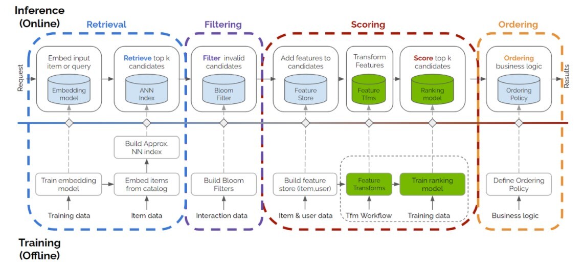
- Retrieval
- Candidate items are generated from the full item catalog, which may be very large. A popular approach to retrieval involves building an embedding model. This is a dense vector space that represents users and items. Approximate Nearest Neighbor (ANN) search is then employed to efficiently retrieve the most suitable candidates.
- Filtering
- Invalid candidates are filtered out. For example, movies that are not suitable for user demographic, such as region and age, availability, or movies that users already watched.
- Scoring
- Valid candidates are scored using a richer set of user, item, and session features and a more expressive model such as a deep neural network.
- Ordering
- A set of top-K candidates are identified. These top-K candidates are reordered according to other business logics and priorities. For example, if there was a marketing campaign for a certain product category or manufacturer, this would be taken into account.
2.2. Components of a Recommender System
Recommender systems contain several key components. As depicted in Figure 2, these components are categorized into four functional areas:
Figure 2. Components of a recommender system
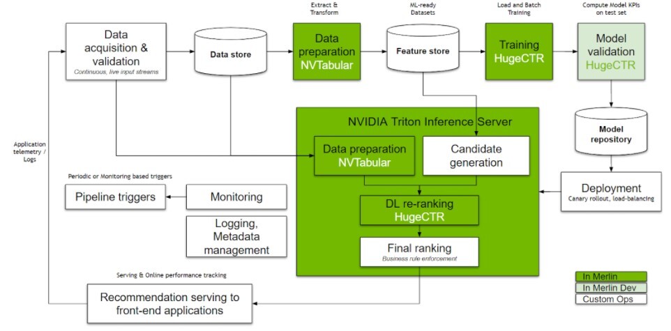
2.2.1. Data Pipeline
The data pipeline contains components for:
2.2.2. Training and Continuous Retraining
Initial training of models takes place so that candidates can be generated and scored. These model candidates are trained on a large amount of available data and deployed. Continuous incremental retraining ensures that the model stays up to date and captures the latest trends and user preferences. A model validation module is used to ensure that the model meets a specified quality threshold.
2.2.3. Deployment and Serving
Newly qualified models are automatically redeployed into production in a seamless manner after initial deployment. This should ideally support canary rollout and rollback. The number of inference servers should also automatically scale up and down as needed.
2.2.4. Logging and Monitoring
Modules are continuously monitored so that the quality of the recommendation can be measured in real time through a range of KPIs, such as hit rate and conversion rate. The modules trigger full retraining should model drift occur, such as when certain KPIs fall below known established baselines.
Data preprocessing and feature engineering play a critical role in building effective machine learning systems. While the advancement of deep learning has lessened the need of manually crafting features in domains such as computer vision and NLP for tabular data, clever feature creation can still have a large impact.
There are a variety of feature engineering techniques that can be leveraged to develop features for recommendation systems, such as multi-modal feature extraction and data augmentation. We have applied and tested these techniques extensively during four recent recommender systems competitions:
3.1. Multi-Modal Feature Extraction Techniques
Aside from tabular data, which is the most popular data source for building recommendation systems, multi-modal data can also be used where possible. Examples include user and product images, free text descriptions, and user text profiles. Features from these modalities can be extracted using domain specific neural networks, such as ResNet for images and BERT for text. These features are then combined with other numerical and categorical features. During the SIGIR eCommerce challenge, we discovered that it was better to apply L2-normalization instead of using the original vectors for the features that are based on text and image. Applying layer normalization individually to each multimodal feature before concatenation with other features improves performance.
3.2. Data Augmentation Techniques
Domain specific data augmentation techniques can be used to enrich the training data. Examples of this include reversing sequences and adding auxiliary data to "non-products".
The goal of the WSDM WebTour Challenge 2021 by Booking.com was to predict the last city destination for a traveler’s trip based on their previous booking history throughout the course of that trip. To augment the data, the trip sequence was reversed, which effectively resulted in twice the amount of training data. Using this approach, NVIDIA data scientists found that the prediction accuracy was improved.
In the SIGIR eCommerce Workshop Challenge 2021 by Coveo, leveraging users’ interactions with "non-product" pages by treating them as a virtual product largely improved our recommendation accuracy. This technique is worth trying for other recommendation problems where page views not associated with items are available.
3.3. Creating and Extracting More Features
Machine learning practitioners have adopted various feature engineering techniques. These feature engineering techniques include the following:
In addition to these feature engineering techniques, domain knowledge should always be leveraged to create features. Examples of this include the extraction of mentions and hashtags in Twitter tweets as they represent entities of special interest.
For the purposes of simplicity, we’re categorizing recommendation models as either traditional machine learning models or deep learning models.
According to the NVIDIA KGMON team, it’s always important to start really simple by using a few features, simple model types, and architectures to develop a baseline, and then add more complex model types and architectures together with additional features.
4.1. Traditional Machine Learning Models
Traditional machine learning models include models such as matrix factorization and gradient boosted models, which are well-proven models that have been deployed widely in production. Tree-based gradient boosted models are high performing models that are often featured in machine learning and recommendation system competitions.
In the Why Are Deep Learning Models Not Consistently Winning Recommender Systems Competitions Yet? research paper, NVIDIA researchers gave an explanation as to why newer deep learning based recommendation models are not consistently winning over traditional machine learning models in public competitions. We can substantiate this claim with our recent RecSys 2020, Recsys 2021, and the Booking.com challenge wins, as well as our second place solution in the SIGIR eCommerce Challenge (Task 2), in which Gradient Boosting Machines (GBM) were featured as an important ingredient. Although deep learning models were also used in these competitions, they don’t completely dominate traditional machine learning models.
4.1.1. Training and Deployment of Tree-Based GBM on GPUs
Popular GBM libraries such as XGboost and LightGB are all accelerated on the GPU. NVIDIA Triton Inference Server FIL Backend allows forest models that are trained by several popular machine learning frameworks, including XGBoost, LightGBM, Scikit-Learn, and cuML, to be deployed in a Triton Inference Server using the RAPIDS Forest Inference Library for fast GPU-based inference. Using this backend, forest models can be deployed seamlessly alongside deep learning models for fast, unified inference pipelines.
4.2. Deep Learning Recommender Models
The increasing availability of large multi-modal datasets in the RecSys domain along with advancements of deep learning within NLP, computer vision, and speech processing has motivated the exploration of deep learning models for building recommender systems in recent years.
Figure 3 depicts the architecture of DLRM (Deep Learning Recommender Model). The inputs to a DLRM can be numerical features or categorical features. Numerical features, such as the number of movies watched, can be directly inputted into MLP layers. However, categorical features, such as country, language, movie title, and genre need to have a numerical representation that can be processed.
Figure 3. Architecture diagram of DLRM
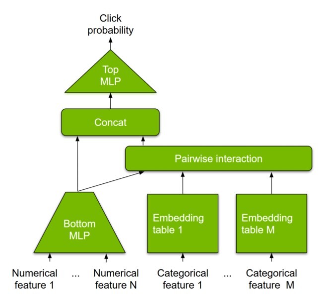
Unlike image or audio data, which are typically numerical and continuous values, the categorical inputs in cases of recommenders are non-numerical and thus require an intermediate processing step to convert them into numerical vectors so that they can be processed. There are two primary ways to do this:
4.2.1. Embeddings
Embeddings are a popular concept in NLP where words/WordPiece tokens are represented numerically through embedding tables. When comparing recommender model embeddings with other types of model embeddings, there are some key differences to note:
About this task
Accessing embeddings often generates a scattered memory access pattern. It is very unlikely that the movies watched will lead to a contiguous access pattern.This can create challenges in memory systems, making them inefficient. NVIDIA GPUs have a highly parallelized memory system that has multiple memory controllers and address translation units, which is great for scattered memory accesses. Additionally, with the latest NVIDIA GPU technology, multi-GPU and multi-node GPU memory capacities are getting sufficiently large for large embeddings. Also, there are methods to leverage CPU memory and/or SSDs/HDDs/NFS through adaptive multi-level storage mechanisms.
4.2.1.1. Batch Sizes and GPU Memory Bandwidth
Since the size of embedding tables depends primarily on the number of distinct categories (vocabulary size) in the feature, the embedding vector size (dimensionality of the embedding vector), and the precision, the embedding table size is calculated as follows:
An embedding table lookup for a one-hot feature operation roughly accesses bytes in memory with embeddings in single-precision.
To generalize it for multi-hot features, and also accounting for any memory used due to index lookup, the memory accessed would be calculated as follows where represents the number of non-zeros or number of entries in the feature field with indices in INT64:
Optimizing GPU memory traffic requires having enough accesses (read/write) in flight at any given time. Based on observation, for smaller batch sizes, higher embedding widths use the GPU memory bandwidth more effectively. For larger batch sizes, the memory traffic saturates as even the narrower width creates enough workload to better utilize it.
Figure 4. GPU memory bandwidth (GB/s) usage for different batch sizes
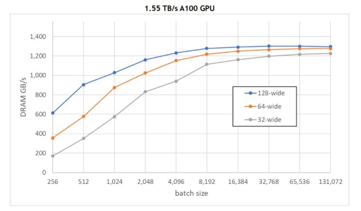
GPU memory bandwidth (GB/s) usage for different batch sizes shows the GPU memory bandwidth (GB/s) usage for different batch sizes using the following experimental settings:
- A100 40 GB GPU with 1.55 TB/s memory bandwidt
- Single embedding table that contains 10M categories tested with three different widths (32, 64, and 128 FP32 elements)
- A single 64-hot, which requires reading 64 vectors, and summing them so that they can be combined
- Embedding table row accesses follow the uniform distribution
Based on GPU memory bandwidth (GB/s) usage for different batch sizes, a batch size of 4K-16K is preferred for one 64-hot table.If N such tables need to be looked up concurrently, the same total memory traffic can be achieved with (batch size / N).This is because the total memory accessed in a batch remains the same. As a best practice, use the largest batch size that allows you to achieve a good enough accuracy to remain efficient.
4.2.1.2. Embedding Width
Embedding width refers to the size (in bytes) of each vector in an embedding table. For example, if each vector in a table has an embedding vector size of 16 and is represented in FP32 precision, the embedding width will be 64 bytes.
It is recommended to pad embedding widths to a multiple of 16 bytes. Typically, multiples of 64 or 128 bytes lead to even better performance.
Based on Figure 5, we see that choosing or padding embedding widths to a multiple of 16 bytes leads to an average performance speedup of 1.05, a maximum performance speedup of 1.26, and a slowdown of 0.97. The larger speedup is seen closer to the edges before the multiple occurs. An example of this would be choosing a width of 32 bytes in place of 31 bytes. The additional capacity may even benefit the model with a better representation.
Figure 5. Benefits of padding embedding widths to a multiple of 16 bytes
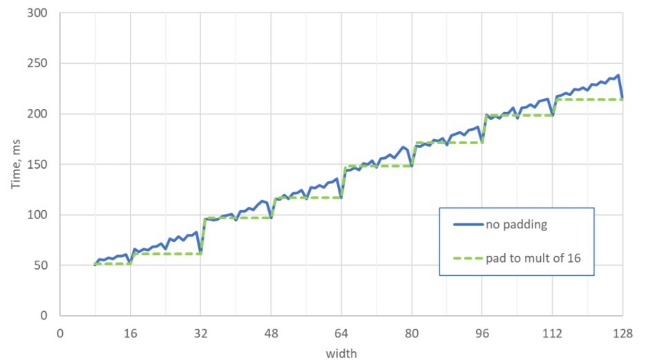
Figure 5 demonstrates the speed of the embedding access operation at different embedding widths using the following experimental settings:
- A100 40 GB GPU with 1.55 TB/s memory bandwidth
- Single embedding table with 10M categories tested for different embedding widths
- A 64-hot, singular feature with a batch size of 8K
- Embedding table row accesses follow the uniform distribution
Using similar experimental settings that were used in Figure 5, if row accesses are distributed according to a power-law distribution, which essentially means that a few rows are accessed very often and many rows are accessed infrequently, an average speedup of 1.03 is observed.
4.2.1.3. Common Practices for Embeddings That Exceed the GPU Memory
In case the size of the embedding tables exceed the memory of a single GPU, these approaches or a combination of these are commonly used in practice:
To support large embeddings, NVIDIA HugeCTR has several best practices baked in by design. HugeCTR, is a GPU-accelerated recommender framework designed to distribute training across multiple GPUs and nodes and estimate Click-Through Rates (CTRs). It also extends it’s functionality for model-parallel training to other frameworks like TensorFlow with it’s Sparse Operation Kit (SOK), which utilizes all available GPUs in both single or multi-node systems for model-parallelism distributed embedding. To learn more about these features, refer to NVIDIA HugeCTR.
4.2.1.4. Fusing Embedding Tables
In recommender models, categorical features need to be embedded to be fed into the MLP layers.
If several embedding tables have the same width (embedding vector size), it can be beneficial to fuse them to create one larger table. This is because frameworks, such as PyTorch and TensorFlow, can have additional overhead for calling embedding lookup individually. As a result, combining tables when possible, unless there is a good reason not to, will give better efficiency in terms of GPU execution and scheduling.
Take a look at the following pseudocode where two tables, embedding1 and embedding2, with the same width are declared and accessed separately.
            # Unfused implementation pseudocode
# declaration
embedding1 = embeddingBag(cardinality_emb_1, vector_dim=128)
embedding2 = embeddingBag(cardinality_emb_2, vector_dim=128)

# Lookup
batch_emb1 = embedding1([list of indices feature 1])
batch_emb2 = embedding2([list of indices feature 2])
As a best practice, fusing the embedding tables to create one larger table leads to better performance.
            # Fused implementation pseudocode
# declaration
embedding12 = embeddingBag(cardinality_emb_1+cardinality_emb_2, vector_dim=128)

# Lookup
new_indices_feature2 = [list of indices feature 2] + cardinality_emb_1
lookup_indices = concat([list of indices feature 1] , new_indices_feature2 )
batch_emb = embedding12([lookup_indices])
4.2.2. MLP Layers
Fully-connected layers typically follow embedding layers in deep learning recommender models and feature crossing layers in some models. The inputs for MLPs include the feature embeddings and numerical features. The output depends on the type of model being trained. In ranking models, the MLPs output a scalar probability, which indicates relevance of the item to the user. Whereas in embedding models, the output may be a vector, which represents the embedding.
Typically, MLPs in recommender ranking models are quite shallow (between 3-5 layers) and often take the shape of a tower as layers get narrower towards the output. For example, N-2048-1024-512-256-1 where N equals all input features combined. However, it is not uncommon to see other topologies like equal width MLPs in which each layer has the same number of nodes, and research indicates that equal width MLPs perform slightly better. Larger batch sizes help saturate the available compute (FLOPs). The following batch sizes are recommended for optimum training:
- 8K-16K for large MLPs such as N-2048-1024-512-256-1
- 32K-64K for smaller MLPs
Figure 6. TFlops and Elapsed Time (ms) compared against batch size for four-layer MLPs with different layer sizes
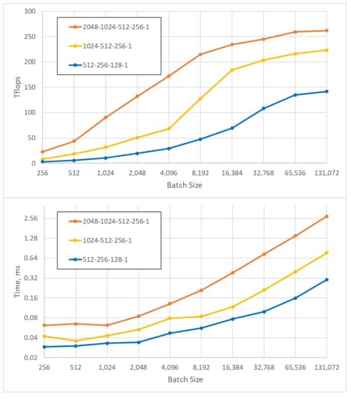
The results depicted in Figure 6 are from a forward pass and MLP layers only, which were tested on an NVIDIA A100 GPU (theoretical peak of 312 dense FP16 TFlops).
In Figure 6, we observe that the elapsed time is roughly flat for the three MLP configurations until the batch size reaches between 2K and 4K. Ranking inference models could work with larger batch sizes without much loss in latency performance in the MLP portion. Ranking models have a higher fidelity than candidate generation models, so keeping everything the same will make it possible to increase the number of candidates generated for a minimal additional cost.
In general, considering both embeddings and MLPs, it can be beneficial to keep the batch size to be 8K or above for optimum training.
4.2.3. Enabling Automatic Mixed Precision
Automatic Mixed precision (AMP) enables training with half precision (FP16) without a loss in network accuracy that is achieved with full precision. Automatic mixed precision reduces training time and memory requirements, enabling higher batch sizes, larger models, and larger inputs. It can deliver up to three times higher training performance than FP32 with a few lines of code, automatically utilizing Tensor Cores in NVIDIA GPUs.
AMP is supported natively in most major Frameworks like PyTorch, TensorFlow, MXNet, and PaddlePaddle. It is recommended to leverage AMP whenever possible.
For more information, refer to our NVIDIA Training With Mixed Precision documentation.
4.2.4. Sequential and Session-Based Recommendation Models
Traditional recommendation algorithms, such as collaborative filtering, usually ignore the temporal dynamics and the sequence of interactions when trying to model user behavior. However, users' preferences do change over time. Sequential recommendation algorithms are able to capture sequential patterns in the users' browsing that might help to predict the users’ interests for better recommendation. For example, users who are starting a new hobby like cooking or cycling might explore products for beginners, and may move to more advanced products over time. They may also completely move on to another hobby of interest. Therefore, recommending items related to their past preferences would become irrelevant.
A special case of sequential-recommendation is the session-based recommendation task where you only have access to the short sequence of interactions within the current session. This is very common for online services like e-commerce, news, and media portals where the user might be brand new or prefers to browse anonymously, and no cookies are collected as a result of the GDPR compliance. This task is also relevant for scenarios where the user’s interests change a lot over time depending on the user’s context or intent, so leveraging the current session interactions is more promising than old interactions to provide relevant recommendations.
To deal with sequential and session-based recommendation, many sequence learning algorithms previously applied in machine learning and NLP research have been explored for RecSys, such as k-Nearest Neighbors, Frequent Pattern Mining, Hidden Markov Models, Recurrent Neural Networks, and more recently neural architectures using the Self-Attention Mechanism and the Transformer architectures.
In our own research at NVIDIA, we found out that Transformer architectures are able to provide more accurate recommendation for sequential and session-based recommendation. We have developed the Transformers4Rec Library, which works as a bridge between Transformer architectures. For more information, refer to the Transformers4Rec: Bridging the Gap between NLP and Sequential / Session-Based Recommendation paper and Transformers4Rec: A Flexible Library for Sequential and Session-based Recommendation article.
Figure 7. Sequential and session-based recommendations with Transformers4Rec
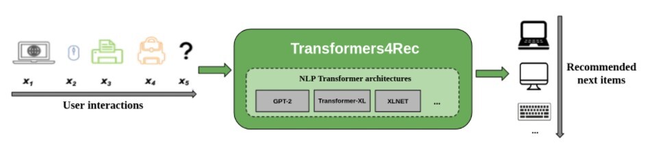
The lessons learned from our extensive empirical analysis that involved benchmarking different algorithms and our recent wins during the following challenges have been applied to the development of the Transformers4Rec Library: Recsys Challenge 2021, WSDM WebTour Challenge 2021 by Booking.com, and SIGIR eCommerce Workshop Challenge 2021 by Coveo. For example, we learned that the XLNet transformer architecture trained with a masked language modeling approach, autoencoding as proposed for BERT, was a top performer across competition and research datasets and would be a good first choice for sequential recommendation problems.
The best practices referenced here will help you build deep learning recommenders using frameworks such as NVIDIA NVTabular, NVIDIA HugeCTR, PyTorch, and TensorFlow.
5.1. NVIDIA NVTabular
NVIDIA NVTabular is a feature engineering and preprocessing library for tabular data. It was designed for quickly and easily manipulating terabyte scale datasets so that deep learning based recommender systems can be trained.
5.1.1. Dataloading
NVIDIA NVTabular provides highly optimized data loaders for training recommender systems in TensorFlow and PyTorch, which reads data directly into the GPU.
5.1.2. Efficient Data Loading with NVIDIA NVTabular
The NVIDIA NVTabular data loader is designed to feed tabular data efficiently to deep learning model training using either PyTorch or TensorFlow. In our experiments, we were able to speed up existing TensorFlow pipelines by nine times and existing PyTorch pipelines by five times with our highly-optimized dataloaders. For more information, refer to Accelerated Training with TensorFlow and Accelerated Training with PyTorch.
5.1.3. Preferred Storage Format
Parquet is the preferred storage format when using NVIDIA NVTabular. It is a compressed tabular data format that is widely used and can be read by libraries like Pandas and CuDF to quickly search, filter, and manipulate data using high level abstractions. NVIDIA NVTabular can read parquet files very quickly.
5.2. NVIDIA HugeCTR
NVIDIA HugeCTR is a high efficiency GPU framework designed for Click-Through-Rate (CTR) estimating training. It provides distributed training with model-parallel embedding tables, embedding cache, and data-parallel neural networks across multiple GPUs and nodes for maximum performance.
5.2.1. Large Embedding Tables
By design, NVIDIA HugeCTR distributes embeddings across multiple GPUs and nodes efficiently for training. For multi-node training, Infiniband with GPU-RDMA support will maximize performance of inter-node transactions. For example, if you have a 1TB embedding table and 16 NVIDIA V100 32 GB GPUs in a server node, you can use two server nodes to fit the table.
NVIDIA HugeCTR also extends it’s functionality to other frameworks like TensorFlow with it’s Sparse Operation Kit, providing an efficient capability for model parallel training to fully utilize all available GPUs in both single-node or multi-node systems. It is also compatible with data parallel training to enable “hybrid parallelism” where the memory intensive embedding parameters can be distributed among all available GPUs, and the MLP layers that are less GPU resource intensive can stay data parallel. For more information, refer to our Sparse Operation Kit documentation.
With its Embedding Training Cache (ETC) feature, NVIDIA HugeCTR can train large models that exceed the available cumulative GPU memory. It does this by dynamically loading a subset of an embedding table into the GPU memory during the training stage, making it possible to train models that are terabytes in size. It supports both single-node/multi-GPU and multi-node/multi-GPU configurations.
5.2.2. Embedding Vector Size
The embedding vector size is related to the size of the Cooperative Thread Array (CTA) for the NVIDIA HugeCTR kernel launch. It should not exceed the maximum number of threads per block (1024 for NVIDIA A100 GPU). Configuring the embedding vector size to a multiple of the warp size (32 threads in a warp for NVIDIA A100 GPU) is recommended to improve occupancy.
5.2.3. Embedding Performance
NVIDIA HugeCTR embedding supports model parallelism where a gigantic embedding table spans multiple GPUs. It implies that inter-GPU communication exists between embedding layers and dense layers with MLPs. To achieve the best performance, we recommend that a NVSwitch equipped machine, such as DGX A100, be used although NVIDIA HugeCTR also works on machines that use NVIDIA Collective Communications Library (NCCL) without NVSwitch.
5.2.4. Data Reader
The NVIDIA HugeCTR data reader is inherently asynchronous and multi-threaded. Users can specify the number of worker threads used to read the dataset. To achieve the best GPU utilization and load balancing, it is recommended that the number of workers be a multiple of the number of GPUs. For instance, if the number of available GPUs is 8, it would be recommended that the number of workers be 8 or 16.
5.3. PyTorch
PyTorch includes several features that can help accelerate training of deep learning based recommender models on NVIDIA GPUs, such as Automatic Mixed Precision and CUDA Graphs.
5.3.1. Using CUDA Graphs
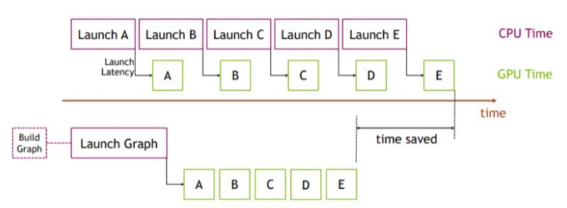
To reduce overhead due to multiple kernel launches, CUDA graphs can be used to cluster a series of CUDA kernels together in a single unit. CUDA graphs were introduced in CUDA 10, and were made available natively in PyTorch v1.10 as a set of beta APIs. For more information about CUDA graphs, refer to the Accelerating PyTorch with CUDA Graphs article, which presents API examples and benchmarks for various models.
The benefits of using CUDA graphs are illustrated in Figure 8 where a CUDA graph is launched in place of a sequence of short kernel launches by the CPU. Initially, a bit more time is used to create and launch the whole graph at once, but overall time is saved due to the minimal gap between kernels.
Figure 8. Time saved by reducing kernel launch overheads with CUDA graphs
In PyTorch, one of the most performant methods to scale out GPU training involves torch.nn.parallel.DistributedDataParallel coupled with the NCCL backend. It applies to both single-node and multi-node distributed training. The CUDA graph benefits mentioned previously also extend to distributed multi-GPU workloads with NCCL kernel launches. Additionally, CUDA graphs establish performance consistency in cases where the kernel launch timings are unpredictable due to various CPU load and operating system factors.
A testament to its performance benefits can be seen in NVIDIA’s MLPerf v1.0 training results where CUDA graphs were instrumental in scaling to over 4000 GPUs, setting new records across the board. For more information, refer to the Global Computer Makers Deliver Breakthrough MLPerf Results with NVIDIA AI blog post.
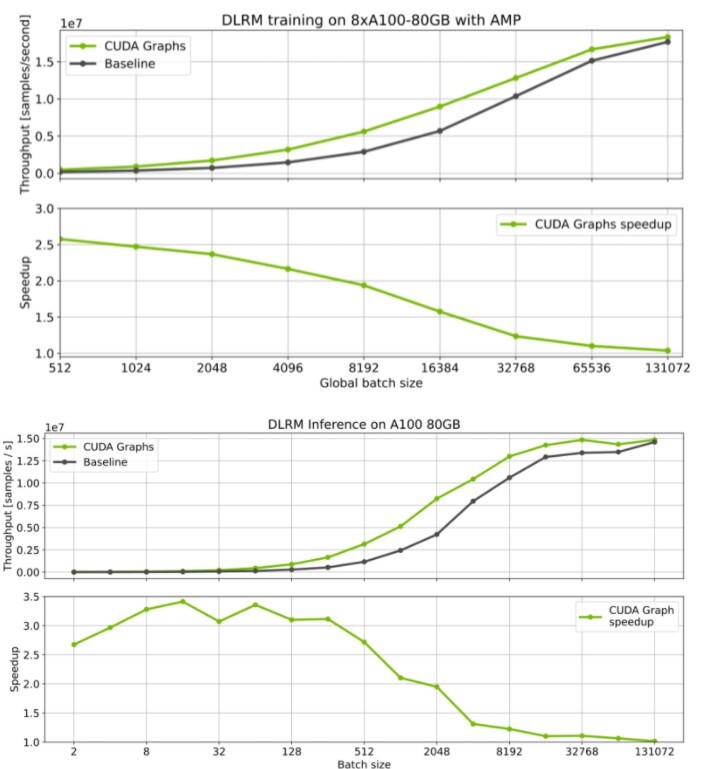
Benchmark results (refer to Figure 9) for NVIDIA’s implementation of the Deep Learning Recommendation Model (DLRM) model show significant speedups for both training and inference. The effects are more visible with small batch sizes where CPU overheads are more pronounced.
Figure 9. Training and inference performance benefits by using CUDA graphs
If you are programming with CUDA or curious about the underlying principles, the CUDA Graphs section of the programming guide and Getting started with CUDA Graphs article are great resources.
5.4. TensorFlow
TensorFlow provides several resources that you can leverage to optimize performance on GPUs. This section contains additional techniques for maximizing deep learning recommender performance on NVIDIA GPUs. For more information about how to profile and improve performance on GPUs, refer to TensorFlow's guide for analyzing and optimizing GPU performance.
5.4.1. I/O Pipeline
TFRecord is a format for storing a sequence of binary records that is preferred by TensorFlow and can be read fast with TensorFlow's native data reader.
Deep learning recommender training is frequently limited by the speed of the data loading as compared to the MLP GEMM compute, which tends to be less time consuming in contrast.
TFRecords store field names along with their values for every example in the data. For tabular data where small float or int features have a smaller memory footprint than string field names, the memory footprint of such a representation can get very big really fast.
5.4.2. Short Field Names
Considering the memory footprint of string field names in TFRecords, a minor optimization could be to keep the field names really short, keeping to the minimum character limit for unique feature names to help improve optimization. This is situational. However, if the data pipeline is limited by disk read speed and the dataset has many small features, this alone can potentially improve the speedup.
5.4.3. Prebatching TFRecords
One way to make data loading faster is by "pre-batching" your data. This means that in each entry (key, value pair) we store a serialized list of values instead to reduce the overhead due to redundant string field names. Therefore, each entry is essentially creating a batch at data preparation time, and we call this "prebatching". The number of values stored in one entry is the "prebatch size".
Figure 10. TFRecord prebatching
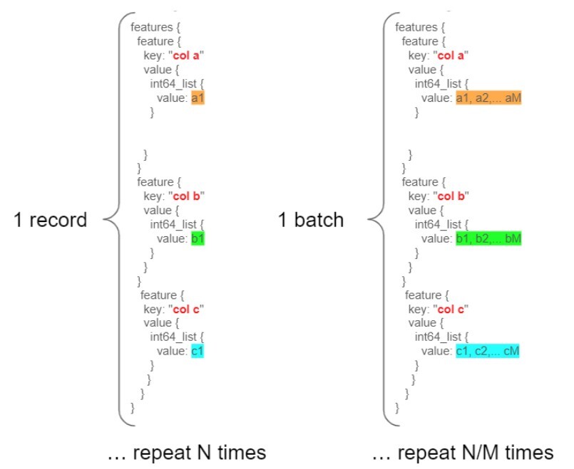
As depicted in Figure 10, let’s use a TFRecord with N entries as an example. Instead of storing each value individually, we serialize M such values for each feature and store the list for each entry. By doing this, we store N/M entries and reduce the overhead due to string field names.
We observe significant speedup at data loading time and overall, which is often the bottleneck in training recommender models on GPUs.
This isn’t without limitations though, and may lead to a loss of some flexibility. You may have to add a component in your data engineering pipeline to create this prebatch, as well as your tf.data pipeline to parse it. Additionally, doing so can limit the ability to shuffle the data, and poses a restriction that the prebatch size is the minimum batch size one can train on. These limitations may or may not be significant depending on the use case.
5.4.4. Grouping Similar Data Types
Along the same lines as prebatching, another option is to group key-value pairs together for the data type.
For example,suppose your data has three categorical features. Instead of having {cat1: [[0]], cat2: [[5]], cat3: [[4]]}, we can store them as {cat: [[0,5,4]]}. The same applies to numerical values. By doing this, we reduce the overhead to store the keys to two strings (one for numeric and one for categorical). However, this may add overhead to keep track of which category is on which index, and would make it more difficult to address multi-hots.
For more information about building performant data input pipelines for training on GPUs, refer to the Tensorflow Performance Guide for tf.data API.
5.4.5. Using XLA Compiler
XLA or Accelerated Linear Algebra is an optimizing compiler for TensorFlow, which supports optimizing code for GPUs. TensorFlow provides documentation to get started with XLA.
NVIDIA’s implementation of the DLRM model also supports XLA JIT compilation. It delivers a steady 10% to 30% performance boost depending on the hardware platform, precision, and the number of GPUs.
5.4.6. Optimized embedding layers
TensorFlow native embedding layers, such as tf.nn.embedding_lookup and tf.nn.embedding_lookup_sparse, do not support model parallelism out of the box, such as distributed embeddings over multiple GPUs or nodes. This limits the size of the embedding tables, imposing a restriction that tables must fit within the memory for one GPU.
To solve this problem, the NVIDIA HugeCTR SOK offers an optimized embedding layer implementation for both TensorFlow 2.x and TensorFlow 1.15. The SOK TensorFlow embedding plugin is designed to work conveniently and seamlessly with TensorFlow as a drop-in replacement for the TensorFlow-native embedding layers. It also offers advanced out of the box features, such as model parallelism, that distributes the embedding tables over multiple GPUs. For more information, refer to our blog and SOK documentation.
Notice
This document is provided for information purposes only and shall not be regarded as a warranty of a certain functionality, condition, or quality of a product. NVIDIA Corporation (“NVIDIA”) makes no representations or warranties, expressed or implied, as to the accuracy or completeness of the information contained in this document and assumes no responsibility for any errors contained herein. NVIDIA shall have no liability for the consequences or use of such information or for any infringement of patents or other rights of third parties that may result from its use. This document is not a commitment to develop, release, or deliver any Material (defined below), code, or functionality.
NVIDIA reserves the right to make corrections, modifications, enhancements, improvements, and any other changes to this document, at any time without notice.
Customer should obtain the latest relevant information before placing orders and should verify that such information is current and complete.
NVIDIA products are sold subject to the NVIDIA standard terms and conditions of sale supplied at the time of order acknowledgement, unless otherwise agreed in an individual sales agreement signed by authorized representatives of NVIDIA and customer (“Terms of Sale”). NVIDIA hereby expressly objects to applying any customer general terms and conditions with regards to the purchase of the NVIDIA product referenced in this document. No contractual obligations are formed either directly or indirectly by this document.
NVIDIA products are not designed, authorized, or warranted to be suitable for use in medical, military, aircraft, space, or life support equipment, nor in applications where failure or malfunction of the NVIDIA product can reasonably be expected to result in personal injury, death, or property or environmental damage. NVIDIA accepts no liability for inclusion and/or use of NVIDIA products in such equipment or applications and therefore such inclusion and/or use is at customer’s own risk.
NVIDIA makes no representation or warranty that products based on this document will be suitable for any specified use. Testing of all parameters of each product is not necessarily performed by NVIDIA. It is customer’s sole responsibility to evaluate and determine the applicability of any information contained in this document, ensure the product is suitable and fit for the application planned by customer, and perform the necessary testing for the application in order to avoid a default of the application or the product. Weaknesses in customer’s product designs may affect the quality and reliability of the NVIDIA product and may result in additional or different conditions and/or requirements beyond those contained in this document. NVIDIA accepts no liability related to any default, damage, costs, or problem which may be based on or attributable to: (i) the use of the NVIDIA product in any manner that is contrary to this document or (ii) customer product designs.
No license, either expressed or implied, is granted under any NVIDIA patent right, copyright, or other NVIDIA intellectual property right under this document. Information published by NVIDIA regarding third-party products or services does not constitute a license from NVIDIA to use such products or services or a warranty or endorsement thereof. Use of such information may require a license from a third party under the patents or other intellectual property rights of the third party, or a license from NVIDIA under the patents or other intellectual property rights of NVIDIA.
Reproduction of information in this document is permissible only if approved in advance by NVIDIA in writing, reproduced without alteration and in full compliance with all applicable export laws and regulations, and accompanied by all associated conditions, limitations, and notices.
THIS DOCUMENT AND ALL NVIDIA DESIGN SPECIFICATIONS, REFERENCE BOARDS, FILES, DRAWINGS, DIAGNOSTICS, LISTS, AND OTHER DOCUMENTS (TOGETHER AND SEPARATELY, “MATERIALS”) ARE BEING PROVIDED “AS IS.” NVIDIA MAKES NO WARRANTIES, EXPRESSED, IMPLIED, STATUTORY, OR OTHERWISE WITH RESPECT TO THE MATERIALS, AND EXPRESSLY DISCLAIMS ALL IMPLIED WARRANTIES OF NONINFRINGEMENT, MERCHANTABILITY, AND FITNESS FOR A PARTICULAR PURPOSE. TO THE EXTENT NOT PROHIBITED BY LAW, IN NO EVENT WILL NVIDIA BE LIABLE FOR ANY DAMAGES, INCLUDING WITHOUT LIMITATION ANY DIRECT, INDIRECT, SPECIAL, INCIDENTAL, PUNITIVE, OR CONSEQUENTIAL DAMAGES, HOWEVER CAUSED AND REGARDLESS OF THE THEORY OF LIABILITY, ARISING OUT OF ANY USE OF THIS DOCUMENT, EVEN IF NVIDIA HAS BEEN ADVISED OF THE POSSIBILITY OF SUCH DAMAGES. Notwithstanding any damages that customer might incur for any reason whatsoever, NVIDIA’s aggregate and cumulative liability towards customer for the products described herein shall be limited in accordance with the Terms of Sale for the product.
Android, Android TV, Google Play and the Google Play logo are trademarks of Google, Inc.
Trademarks
NVIDIA, the NVIDIA logo, CUDA, Merlin, RAPIDS, Triton Inference Server, Turing and Volta are trademarks and/or registered trademarks of NVIDIA Corporation in the United States and other countries. Other company and product names may be trademarks of the respective companies with which they are associated.