Is this page helpful?

Working with Quantized Types#

TensorRT enables high-performance inference by supporting quantization, a technique that reduces model size and accelerates computation by representing floating-point values with lower-precision data types.

Key Benefits: - Reduces memory footprint - Improves energy efficiency - Enables deployment on resource-constrained edge devices - Achieves greater cost-efficiency in large-scale data center deployments

Quantization Approach: TensorRT uses a symmetric quantization scheme, where both activations and weights are mapped to quantized values centered around zero. This approach simplifies the transformation between quantized and floating-point representations, typically involving only a scaling factor.

Supported Data Types:

INT8 (signed 8-bit integer)
INT4 (signed 4-bit integer, weight-only quantization)
FP8E4M3 (FP8, 8-bit floating point with 4 exponent and 3 mantissa bits)
FP4E2M1 (FP4, 4-bit floating point with 2 exponent and 1 mantissa bit)

These low-precision formats allow TensorRT to deliver efficient inference while maintaining accuracy, making it suitable for deployment in resource-constrained environments and high-throughput applications.

Quantization Workflows#

TensorRT supports both post-training quantization (PTQ) and quantization-aware training (QAT) workflows. These workflows enable you to optimize models for low-precision data types.

The quantization process uses per-tensor, per-channel, or block-wise scaling. The scaling method depends on the layer and data type, which helps preserve model accuracy during conversion.

Post-Training Quantization (PTQ): - Quantizes a pre-trained model without retraining - Requires representative “calibration data” set to compute quantization parameters - Practical when retraining is infeasible due to resource limitations or data privacy concerns - Can lead to accuracy degradation for complex models or sensitive layers

Quantization-Aware Training (QAT): - Simulates quantization during training by quantizing weights and activation layers - Training actively compensates for quantization and dequantization effects - Generally achieves superior accuracy recovery compared to PTQ - More time-consuming and requires access to the entire labeled training dataset

The TensorRT Model Optimizer is a Python toolkit designed to help you create QAT models. These models are fully compatible with TensorRT’s optimization and deployment workflows.

The toolkit also provides a PTQ recipe that lets you perform PTQ on models developed in both PyTorch and ONNX formats, streamlining the quantization process across different frameworks.

Explicit Quantization Overview#

A TensorRT network is explicitly quantized when it contains Quantize and Dequantize layers (Q/DQ for short), which mark exactly where conversions to and from a quantized type occur. The optimizer performs only the conversions dictated by the semantics of the model.

In explicitly quantized networks, the quantization and dequantization operations are represented by IQuantizeLayer (C++, Python) and IDequantizeLayer (C++, Python) nodes in the graph - these will henceforth be referred to as Q/DQ nodes. IDynamicQuantizeLayer extends this API for Dynamic Quantization workflows where scales are computed at inference time.

ONNX uses an explicitly quantized representation: when a model in PyTorch or TensorFlow is exported to ONNX, each fake-quantization operation in the framework’s graph is exported as a Quantize node followed by a Dequantize node. Since TensorRT preserves the semantics of these layers, users can expect accuracy that is very close to that seen in the deep learning framework. While optimizations preserve the arithmetic semantics of quantization and dequantization operators, they can change the order of floating-point operations in the model, so results will not be bitwise identical.

Key Capabilities:

Broad Data Type Support: Supports INT8, FP8, INT4, and FP4 quantized data types.
Precise Placement Control: Q/DQ nodes specify exactly where conversions to and from quantized types occur, so the optimizer applies only the conversions dictated by the model’s semantics.
Compatibility with ONNX Export: Performing QAT or PTQ in a deep learning framework and exporting to ONNX naturally produces an explicitly quantized model, because ONNX represents fake-quantization operations as Q/DQ pairs.

Calibration is performed before ONNX export (for example, during PTQ or QAT with Model Optimizer), and the resulting scales are embedded directly into the Q/DQ nodes.

Quantization Granularities#

Quantization granularity refers to how quantization scale factors are applied across a model’s tensors. Selecting the appropriate granularity is a direct lever for balancing the benefits of quantization (such as memory reduction) against its potential drawbacks (such as accuracy loss). A more granular approach increases potential accuracy but also increases the computational and memory overhead of managing multiple scaling factors. TensorRT supports three quantization scale granularities:

Per-tensor quantization: a single scale value (scalar) is used to scale the entire tensor.
Per-channel quantization: a scale tensor is broadcast along the given axis - for convolutional neural networks, this is typically the channel axis.
Block quantization: the tensor is divided into fixed-size blocks, and a scale factor is defined for each block. IQuantizeLayer and IDequantizeLayer support 1D block shapes (along a single dimension). For 2D block shapes (along the last two dimensions), use IDynamicQuantizeLayer.

When using per-channel quantization with Convolutions, the quantization axis must be the output-channel axis. For example, when the weights of 2D convolution are described using KCRS notation, K is the output-channel axis, and the weights quantization can be described as:

For each k in K:
    For each c in C:
        For each r in R:
            For each s in S:
                output[k,c,r,s] := clamp(round(input[k,c,r,s] / scale[k]))

The scale is a vector of coefficients and must have the same size as the quantization axis.

Dequantization is performed similarly except for the pointwise operation that is defined as:

output[k,c,r,s] := input[k,c,r,s] * scale[k]

Block Quantization

In block quantization, elements are grouped into blocks, with all elements in a block sharing a common scale factor. Block quantization is supported for inputs of up to 3 dimensions.

INT4 block quantization supports weight-only quantization (WoQ).

FP4 block quantization supports both weights and activations. To minimize quantization error, use Dynamic Quantization for activations.

When using block quantization, the scale tensor dimensions equal the data tensor dimensions except for one dimension over which blocking is performed (the blocking axis). For example, given a 2-D RS weights input, R (dimension 0) as the blocking axis and B as the block size, the scale in the blocking axis is repeated according to the block size and can be described like this:

For each r in R:
    For each s in S:
        output[r,s] = clamp(round(input[r,s] / scale[ceil(r//B), s]))

The scale is a 2D array of coefficients with dimensions (ceil(R//B), S).

Dequantization is performed similarly, except for the pointwise operation that is defined as:

output[r,s] = input[r,s] * scale[ceil(r//B), s]

Quantized Types Rounding Modes#

TensorRT primarily uses the round-to-nearest-even method (also known as “banker’s rounding”), which rounds ties to the nearest even value. For example, 2.5 rounds to 2 and 3.5 rounds to 4. This method helps reduce systematic bias in the quantization process, preventing the consistent upward or downward drift that can occur with other rounding strategies.

For more information about rounding modes, refer to Rounding.

Dynamic Quantization#

Dynamic Quantization is a form of quantization in which the scales are computed during inference according to the input data. It produces two outputs: quantized data and scales. TensorRT supports Dynamic Quantization only with block quantization granularity.

Dynamic Quantization has two main benefits:

Accuracy: With Dynamic Quantization, TensorRT selects a scale that maps only the dynamic range of a single block to the quantized type. Because the dynamic range of a single block is often much smaller than the dynamic range of the entire tensor, the quantization error is reduced. This is most significant for sub-byte quantized types because of the small range of values representable in these data types.
Reduced PTQ overhead: Because TensorRT computes the scales automatically during inference, you don’t need to calibrate them using sample data.

For each block, the scale is computed by:

${scale}=max_{i\in \left\{ 0...blockSize-1 \right\}}\left( \frac{abs\left( x_{i} \right)}{qTypeMax} \right)$

Where:

${qTypeMax}$ is the maximum value in the quantized type (such as 6 for FP4E2M1).

MX-Compliant Dynamic Quantization#

Dynamic Quantization according to the OCP Microscaling Formats (MX) Specification v1.0. The MX-Compliant recipe performs block quantization, quantizing across 32 high-precision elements to produce 32 quantized output values and one E8M0 scaling factor.

TensorRT currently supports MX-Compliant Dynamic Quantization only for the FP8E4M3 vector format, referred to as MXFP8.

The scale computation for a single block is defined as:

$scale_{E8M0}=round\_up\_to\_e8m0\left( max_{i\in \left\{ 0...blockSize-1 \right\}}\left( \frac{abs\left( x_{i} \right)}{qTypeMax} \right) \right)$

Where:

$E8M0$ is an 8-bit exponent-only floating point type, as described in Supported Types.
$round\_up\_to\_e8m0$ is the computed scale rounded up to the smallest power of two that is greater than or equal to it.
$qTypeMax$ is the maximum value representable in the quantized type used for data.

The scale computation is repeated for each block, computing a total of $\frac{inputVolume}{blockSize}$ block scales.

Dynamic Double Quantization#

A variant of Dynamic Quantization, in which the computed scales are also quantized. Putting together the scale computation and scale quantization for a single block:

$scale_{quantized}=quantize\left( max_{i\in \left\{ 0...blockSize-1 \right\}}\left( \frac{abs\left( x_{i} \right)}{qTypeMax} \right), scale=globalSf \right)$

Where:

$globalSf$ is an offline-calibrated per-tensor quantization scale (scalar).

TensorRT currently supports Dynamic Double Quantization only for the NVFP4 vector format (FP4E2M1 data, FP8E4M3 scales, block size of 16).

Using $qTypeMax=6$ and the FP8 range of [-448,448], the quantized scale can be written as:

$scale_{fp8}=castToFp8\left( \frac{max_{i\in \left\{ 0...blockSize-1 \right\}}\left( ^{abs\left( x_{i} \right)} \right)}{6^{\ast }globalSf} \right)$

The quantized data is computed using block quantization and the computed scales.

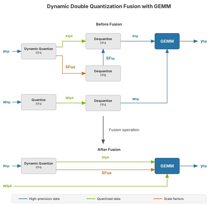
To dequantize data that was quantized using Dynamic Double Quantization, two consecutive Dequantize operations are required (which is why it’s called double quantization): the first dequantizes the scales using per-tensor quantization, and the second dequantizes the data.

$data_{DQ}=dequantize\left( data_{Q},dequantize\left( scale_{Q},scale=globalSf \right) \right)$

Quantization Schemes#

INT8

INT8 quantization and dequantization operations are defined as follows:

$x_{q}=quantize\left(x, s \right)=roundWithTiesToEven(clip(\frac{x}{s}, -128,127))$

${x}=dequantize\left(x_{q}, s\right)=x_{q}\ast s$

Where:

${x}$ is a high-precision floating point value to be quantized.
$x_{q}$ is a quantized INT8 value in range [-128,127].
${s}$ is the quantization scale expressed using a 16-bit or 32-bit floating point scalar.
${roundWithTiesToEven}$. Refer to Rounding.

FP8

FP8 quantization and dequantization operations are defined as follows:

$x_{q}=quantize\left(x, s \right)=castToFp8(clip(\frac{x}{s}, -448,448))$

${x}=dequantize\left(x_{q}, s\right)=x_{q}\ast s$

Where:

${x}$ is a high-precision floating point value to be quantized.
$x_{q}$ is a quantized FP8E4M3 value in the range [-448, 448].
${s}$ is the quantization scale expressed using a 16-bit or 32-bit floating point scalar.
${castToFp8}$ rounds to the nearest value representable in FP8E4M3, ties are rounded to an even number. Refer to Rounding.

MXFP8

MXFP8 is a dynamic per-block quantization scheme. The output type is FP8E4M3, the scale type is E8M0, and the block size is 32. The quantization and dequantization formulas are identical to the FP8 quantization scheme.

When quantizing activations, Dynamic Quantization is required.

INT4

INT4 quantization and dequantization operations are defined as follows:

$x_{q}=quantize\left(x, s \right)=roundWithTiesToEven(clip(\frac{x}{s}, -8,7))$

${x}=dequantize\left(x_{q}, s\right)=x_{q}\ast s$

Where:

${x}$ is a high-precision floating point value to be quantized.
$x_{q}$ is a quantized INT4 value in the range [-8, 7].
${s}$ is the block’s quantization scale expressed using a 16-bit or 32-bit floating point.
${roundWithTiesToEven}$. Refer to Rounding.

INT4 quantization requires per-block scales. The supported block sizes are {64, 128}. The block dimension should be one of the last two dimensions.

TensorRT only supports INT4 for weight quantization (Q/DQ Layer-Placement Recommendations).

NVFP4

NVFP4 quantization requires per-block scales. The only supported block size is 16. The block dimension should be one of the last two dimensions.

$x_{q}=quantize\left(x, s \right)=castToFp4(clip(\frac{x}{s}, -6,6))$

${x}=dequantize\left(x_{q}, s\right)=x_{q}\ast s$

Where:

${x}$ is a high-precision floating point value to be quantized.
$x_{q}$ is a quantized FP4 value in the range [-6, 6].
${s}$ is the block’s quantization scale expressed using a 16-bit or 32-bit floating point.
${castToFp4}$ rounds to the nearest value representable in FP4E2M1, ties are rounded to an even number. Refer to Rounding.

When quantizing activations, Dynamic Quantization is required.

Table 10 Quantization Schemes and Precision#
Quantization Schemes	INT8	FP8	MXFP8	INT4	NVFP4
Representation	8-bit signed 2’s complement	S1E4M3 floating point	S1E4M3 floating point	4-bit signed 2’s complement	S1E2M1 floating point
Weight quantization	Per-tensor/per-axis	Per-tensor/per-axis	Per-block (block size = 32)	Per-block (block sizes = `{64, 128}`)	Per-block
Activation quantization	Per-tensor	Per-tensor	Dynamic, per-block (block size = 32)	No	Dynamic, per-block
Explicit quantization	Yes	Yes	Yes	Yes	Yes
Scale data type	FP32, FP16, BF16	FP32, FP16, BF16	E8MO	FP32, FP16, BF16	FP32, FP16, BF16

Explicit Quantization#

When TensorRT detects Q/DQ layers in a network, it builds an engine using explicit quantization processing logic. The rest of this section describes how explicit quantization operates in more detail.

Use explicit quantization with Strong Typing. Precision-control build flags are not required and should not be specified.

Quantized Weights#

You can specify weights of Q/DQ models using a high-precision data type (FP32, FP16, or BF16) or a low-precision quantized type (INT8, FP8, INT4, or FP4). When TensorRT builds an engine, it quantizes high-precision weights using the IQuantizeLayer scale, which operates on the weights. The quantized (low-precision) weights are stored in the engine plan file. When using pre-quantized weights, an IDequantizeLayer is required between the weights and the linear operator that uses them.

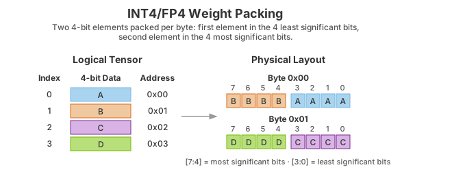
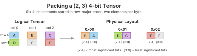
INT4 and FP4 quantized weights are stored by packing two elements per byte. The first element is stored in the 4 least significant bits, and the second is stored in the 4 most significant bits.

4-bit packing (logical tensor on the left; physical layout on the right)

The following example illustrates this packing for a (2, 3) tensor.

ONNX Support#

When a model trained in PyTorch or TensorFlow using quantization-aware training (QAT) is exported to ONNX, each fake-quantization operation in the framework’s graph is exported as a pair of QuantizeLinear and DequantizeLinear ONNX operators. When TensorRT imports an ONNX model, the ONNX QuantizeLinear operator is imported as an IQuantizeLayer instance, and the ONNX DequantizeLinear operator is imported as an IDequantizeLayer instance.

ONNX introduced support for QuantizeLinear and DequantizeLinear in opset 10, and a quantization-axis attribute was added in opset 13 (required for per-channel quantization). PyTorch 1.8 introduced support for exporting PyTorch models to ONNX using opset 13.

ONNX opset 19 added four FP8 formats, of which TensorRT supports E4M3FN (also referred to as tensor (float8e4m3fn) in the ONNX operator schema). The latest PyTorch version (PyTorch 2.0) does not support FP8 formats, nor does it support exporting to ONNX using opset 19. To bridge the gap, TransformerEngine exports its FP quantization functions as custom ONNX Q/DQ operators that belong to the “trt” domain (TRT_FP8 QuantizeLinear and TRT_FP8 DequantizeLinear). TensorRT can parse both the custom operators and standard opset 19 Q/DQ operators. Note that TensorRT does not fully support opset 19, and other tools such as ONNX Runtime cannot parse the custom operators. ONNX opset 21 added support for the INT4 data type and block quantization, and ONNX opset 23 added support for the FP4E2M1 type.

Warning

The ONNX GEMM operator is an example that can be quantized per channel. PyTorch torch.nn.Linear layers are exported as an ONNX GEMM operator with (K, C) weights layout and the transB GEMM attribute enabled, which transposes the weights before performing the GEMM operation. TensorFlow, on the other hand, pre-transposes the weights (C, K) before ONNX export:

PyTorch: $y=xW^{T}$
TensorFlow: $y=xW$

TensorRT, therefore, transposes PyTorch weights. TensorRT quantizes the weights before they are transposed, so GEMM layers originating from ONNX QAT models that were exported from PyTorch use dimension 0 for per-channel quantization (axis K = 0), while models originating from TensorFlow use dimension 1 (axis K = 1).

TensorRT does not support pre-quantized ONNX models that use INT8 or FP8 quantized operators. Specifically, the following ONNX quantized operators are not supported and generate an import error when TensorRT encounters them while importing the ONNX model:

QLinearConv and QLinearMatmul
ConvInteger and MatmulInteger

TensorRT Processing of Q/DQ Networks#

When TensorRT optimizes a network in Q/DQ mode, the optimization process is limited to optimizations that do not change the arithmetic correctness of the network. Bit-level accuracy is rarely possible because the order of floating-point operations can produce different results. For example, rewriting ${a}\ast s+b\ast s$ as $\left(a+b \right)\ast s$ is a valid optimization. Allowing these differences is fundamental to backend optimization in general, and the same applies to converting a graph with Q/DQ layers to use quantized operations.

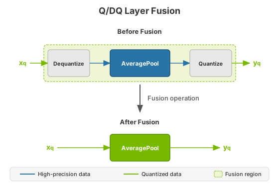
Q/DQ layers control the compute and data precision of a network. An IQuantizeLayer instance converts a high-precision floating-point tensor to a quantized tensor, and an IDequantizeLayer instance converts a quantized tensor back to a high-precision floating-point tensor. TensorRT expects a Q/DQ layer pair on each input of quantizable layers. Quantizable layers are deep-learning layers that can be converted to quantized layers by fusing with IQuantizeLayer and IDequantizeLayer instances. When TensorRT performs these fusions, it replaces the quantizable layers with quantized layers that operate on quantized data using compute operations suitable for quantized types.

A quantizable ``AveragePool`` layer (in blue) is fused with the surrounding Dequantize and Quantize layers. All three layers are replaced by a single quantized ``AveragePool`` layer (in green).

During network optimization, TensorRT moves Q/DQ layers in a process called Q/DQ propagation. The goal of propagation is to maximize the proportion of the graph that can be processed at low precision. To achieve this, TensorRT propagates Quantize nodes backward (so quantization happens as early as possible) and Dequantize nodes forward (so dequantization happens as late as possible). Quantize layers can swap places with layers that commute with quantization, and Dequantize layers can swap places with layers that commute with dequantization.

A layer ${Op}$ commutes with quantization if ${Q}\left(Op\left(x \right) \right)=={Op}\left(Q\left(x \right) \right)$

Similarly, a layer ${Op}$ commutes with dequantization if ${Op}\left(DQ\left(x \right) \right)=={DQ}\left(Op\left(x \right) \right)$

The following diagram illustrates Dequantize forward propagation and Quantize backward propagation. These are legal rewrites of the model because Max Pooling has an INT8 implementation and commutes with both Dequantize and Quantize.

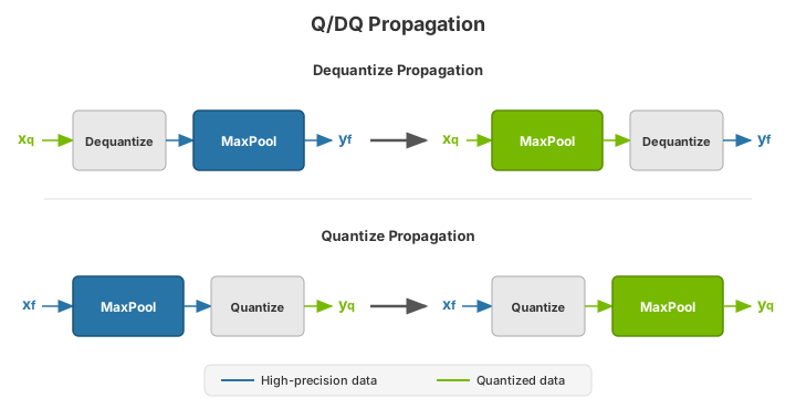
An illustration of Dequantize forward-propagation and Quantize backward-propagation through a Max Pooling layer.

To understand Max Pooling commutation, let us look at the output of the maximum-pooling operation applied to some arbitrary input. Max Pooling is applied to groups of input coefficients and outputs the coefficient with the maximum value. For group i composed of coefficients $\left\{x_{0}..x_{m} \right\}$:

$output_{i}:=max\left( \left\{ x_{0},x_{1},...x_{m} \right\} \right)=max\left( \left\{max\left( \left\{ max\left( \left\{ x_{0},x_{1} \right\} \right),x_{2} \right\} \right),...x_{3} \right\} \right)$

It is, therefore, enough to look at two arbitrary coefficients without loss of generality (WLOG):

$x_{j}=max\left( \left\{ x_{j},x_{k} \right\} \right)for\: x_{j}\ge x_{k}$

For the quantization function ${Q}\left( a,scale,x_{max},x_{min} \right):=truncate\left( round\left( \frac{a}{scale} \right),x_{max},x_{min}\right) scale> 0$, note that (without providing proof and using simplified notation): ${Q}\left( x_{j},scale \right)\ge {Q}\left( x_{k},scale \right)for x_{j}\ge x_{k}$

Therefore: ${max}\left( \left\{ {Q}\left( x_{j},scale \right),{Q}\left( x_{k},scale \right) \right\} \right)={Q}\left( x_{j},scale \right) for x_{j}\ge x_{k}$

However, by definition: ${Q}\left( max\left( \left\{ x_{j},x_{k} \right\} \right),scale \right)={Q}\left( x_{j},scale \right) for x_{j}\ge x_{k}$

Function ${max}$ commutes with quantization, and so does Max Pooling.

Similarly, for dequantization, function ${DQ}\left( a,scale \right):=a\ast scale$ with ${scale}> 0$ it can be shown that: ${max}\left( \left\{ {DQ}\left(x_{j},scale \right),{DQ}\left( x_{k},scale \right) \right\} \right)={DQ}\left( x_{j},scale \right)={DQ}\left( {max}\left( \left\{ x_{j},x_{k} \right\} \right),scale \right) for x_{j}\ge x_{k}$

There is a distinction between how quantizable layers and commuting layers are processed. Both kinds of layers can be computed in INT8 or FP8, but quantizable layers also fuse with a Dequantize input and a Quantize output. For example, an AveragePooling layer (quantizable) does not commute with either Quantize or Dequantize, so it is quantized using Q/DQ fusion, as shown in the first diagram. This is in contrast to how Max Pooling (commuting) is quantized.

Weight-Only Quantization#

Weight-only quantization (WoQ) is an optimization useful when memory bandwidth limits the performance of GEMM operations or when GPU memory is scarce. In WoQ, GEMM weights are quantized to INT4 precision while the GEMM input data and compute operation remain in high precision. TensorRT’s WoQ kernels read the 4-bit weights from memory and dequantize them before performing the dot product in high precision.

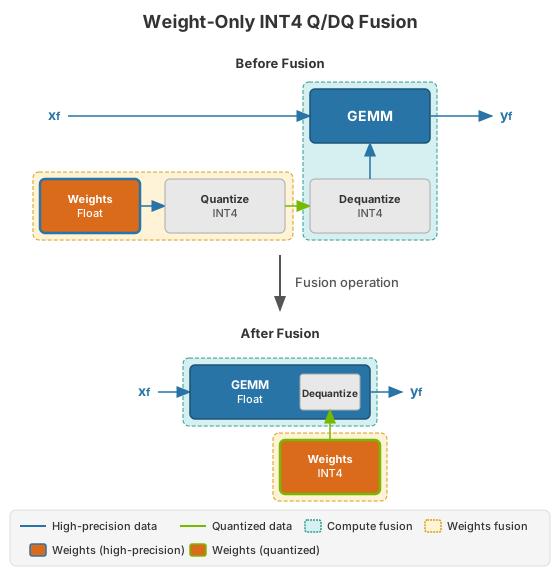
WoQ is available only for INT4 block quantization with GEMM layers. The GEMM data input is specified in high precision (FP32, FP16, or BF16), and the weights are quantized using Quantize and Dequantize layers as usual. TensorRT creates an engine with INT4 weights and a high-precision GEMM operation. The engine reads the low-precision weights and dequantizes them before performing the GEMM operation in high precision.

Q/DQ Layer-Placement Recommendations#

The placement of Q/DQ layers in a network affects performance and accuracy. Aggressive quantization can degrade model accuracy because quantization introduces error, but quantization also reduces latency. The following recommendations help you place Q/DQ layers effectively in your network.

Older devices might not have low-precision kernel implementations for all layers, and you can encounter a could not find any implementation error while building your engine. To resolve this, remove the Q/DQ nodes that quantize the failing layers.

Quantize all inputs of weighted operations (Convolution, Transposed Convolution, and GEMM). Quantizing the weights and activations reduces bandwidth requirements and enables INT8 computation to accelerate bandwidth-limited and compute-limited layers.

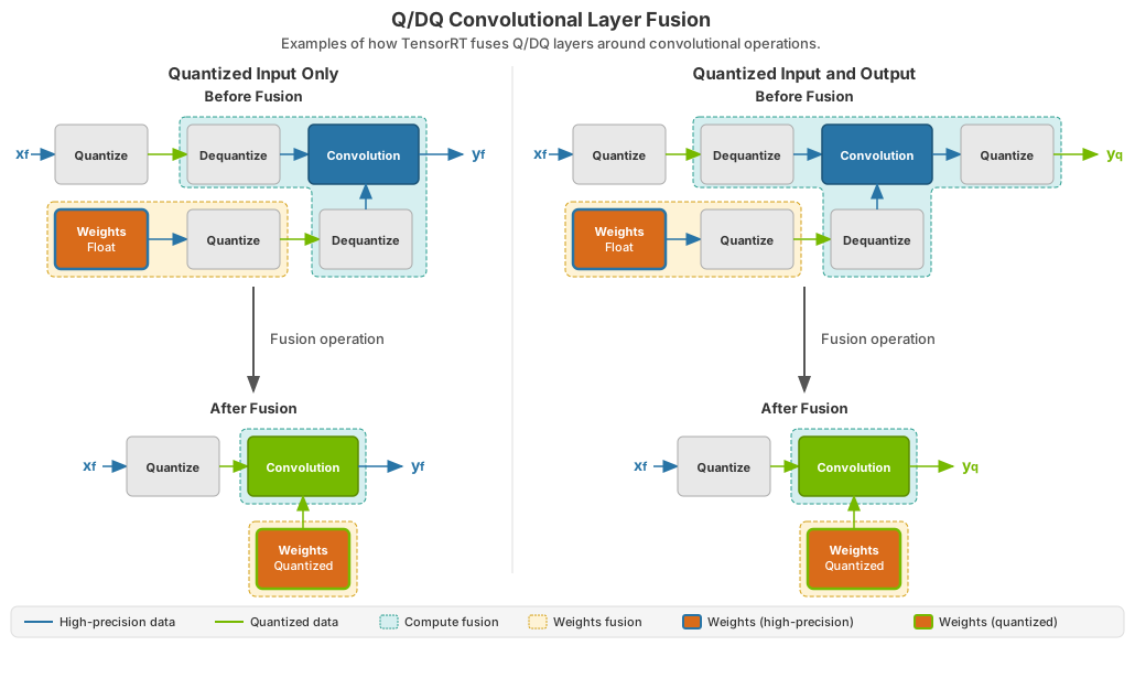
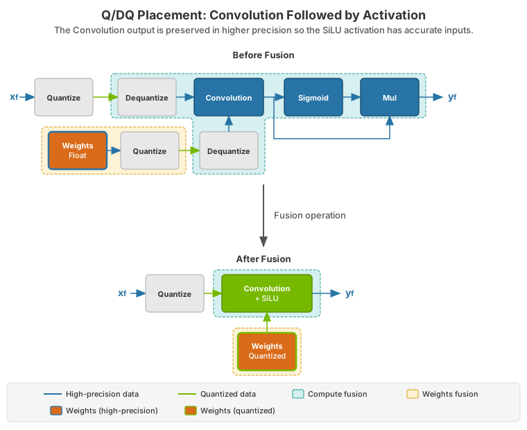
By default, do not quantize the outputs of weighted operations. It is sometimes useful to preserve the higher-precision dequantized output. For example, if the linear operation is followed by an activation function (SiLU, in the following diagram), the activation requires higher-precision input to produce acceptable accuracy.

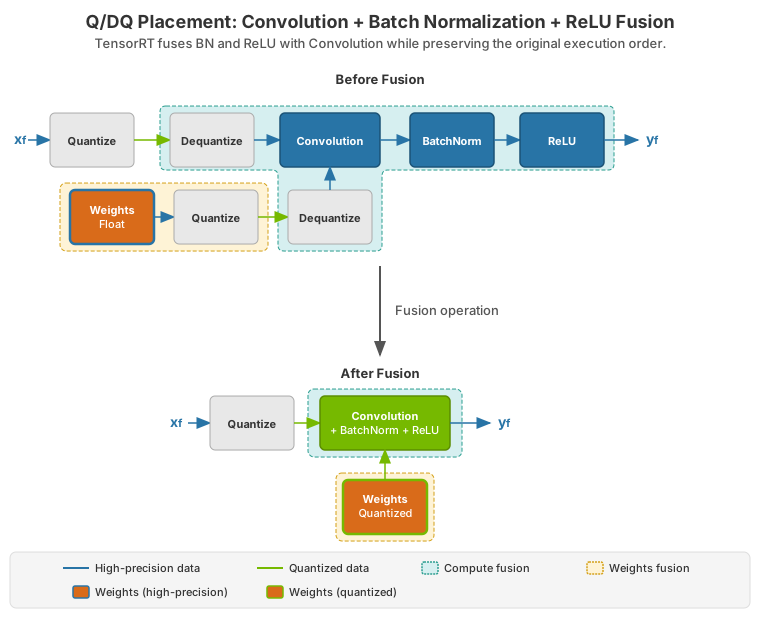
Do not simulate batch normalization and ReLU fusions in the training framework because TensorRT optimizations guarantee the preservation of these operations’ arithmetic semantics.

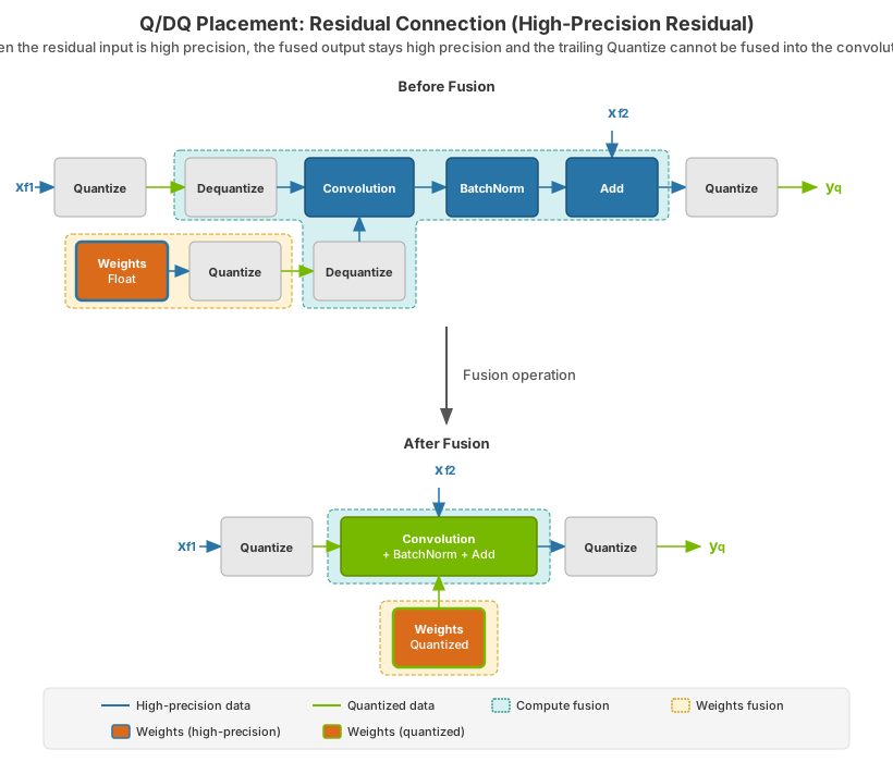
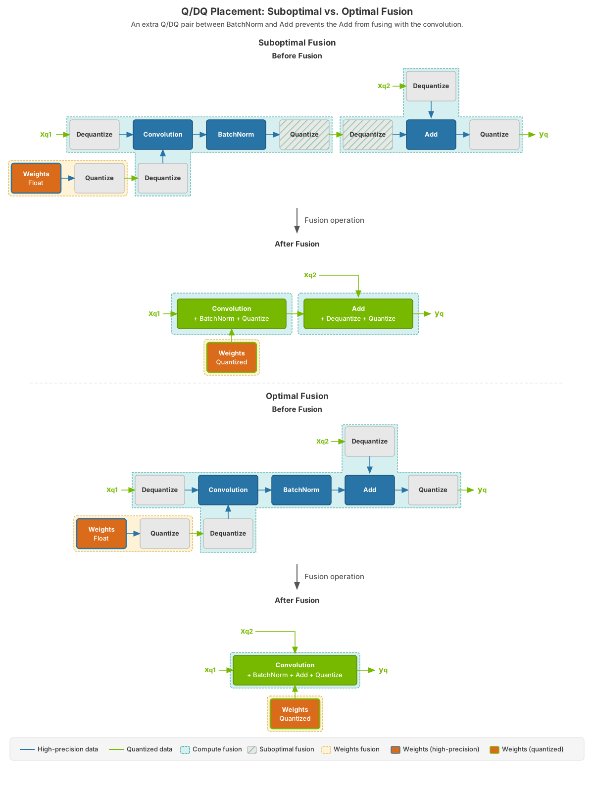
Quantize the residual input in skip connections. TensorRT can fuse element-wise addition following weighted layers, which is useful for models with skip connections like ResNet and EfficientNet. The precision of the first input to the element-wise addition layer determines the fusion output’s precision.

For example, in the following diagram, the precision of $x_{f^{}}^{2}$ is high precision, so the output of the fused convolution is limited to high precision, and the trailing Q-layer cannot be fused with the convolution.

$:math:`x_{f^{}}^{2}` is high precision, so the output of the fused convolution is limited to high precision, and the trailing Quantize layer cannot be fused with the convolution.$

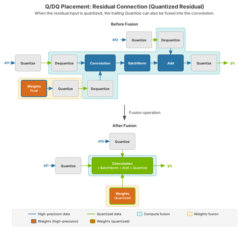
In contrast, when $x_{f^{}}^{2}$ is quantized to INT8, as depicted in the following diagram, the output of the fused convolution is also INT8, and the trailing Q-layer is fused with the convolution.

$When :math:`x_{f^{}}^{2}` is quantized to INT8, the output of the fused convolution is also INT8, and the trailing Quantize layer is fused with the convolution.$

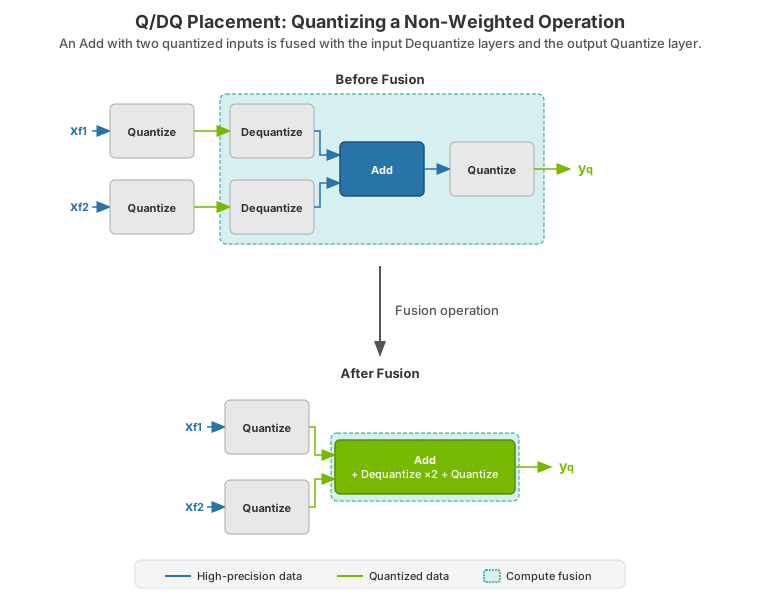
For extra performance, try quantizing layers that do not commute with Q/DQ. Currently, non-weighted layers with INT8 inputs also require INT8 outputs, so quantize both inputs and outputs.

Performance can decrease if TensorRT cannot fuse the operations with the surrounding Q/DQ layers, so be conservative when adding Q/DQ nodes and experiment with both accuracy and TensorRT performance in mind.

The following figure contrasts a suboptimal Q/DQ placement against an optimal one for a convolution followed by an element-wise addition.

Use per-tensor quantization for activations and per-channel quantization for weights. This configuration has been demonstrated empirically to lead to the best quantization accuracy.

You can further optimize engine latency by enabling FP16. TensorRT attempts to use FP16 instead of FP32 whenever possible (this is not currently supported for all layer types).

Q/DQ Limitations#

Some of the Q/DQ graph-rewrite optimizations that TensorRT performs compare the quantization scales of two or more Q/DQ layers and only apply the rewrite when those scales are equal. When you refit a refittable TensorRT engine, the scales of Q/DQ nodes can be assigned new values. During refitting, TensorRT checks whether any Q/DQ layers that participated in scale-dependent optimizations have new values that break those rewrites. If they do, TensorRT throws an exception.

Q/DQ Interaction with Plugins#

Plugins extend TensorRT’s capabilities by allowing the replacement of a group of layers with a custom and proprietary implementation. You can decide what functionality to include in the plugin and what to leave for TensorRT to handle.

The same applies to a TensorRT network with Q/DQ layers. When a plugin consumes quantized inputs (INT8/FP8) and generates quantized outputs, the input Dequantize and output Quantize nodes must be included in the plugin and removed from the network.

Consider a simple case of a sequential graph consisting of a single INT8 plugin (aptly named MyInt8Plugin) sandwiched between two convolution layers (ignoring weights quantization):

${Input}> {Q}\rightarrow {DQ}> {Conv}> {Q}\rightarrow {DQ\_i}> {MyInt8Plugin}> {Q\_o}\rightarrow {DQ}> {Conv}> {Output}$

The $>$ arrows indicate activation tensors with FP32 precision, and the $\rightarrow$ arrows indicate INT8 precision.

When TensorRT optimizes this graph, it fuses the layers to the following graph (square brackets indicate TensorRT fusions):

${Input}> {Q}\rightarrow \left[{DQ}\rightarrow {Conv}\rightarrow {Q}\right]\rightarrow {DQ\_i}> {MyInt8Plugin}> {Q\_o}\rightarrow \left[{DQ}\rightarrow {Conv}\right]> {Output}$

In the graph above, the plugin consumes and generates FP32 inputs and outputs. Because the plugin MyInt8Plugin uses INT8 precision, you must manually integrate $DQ\_i$ and $Q\_o$ into the plugin and then call setOutputType(kINT8) for that plugin layer. TensorRT then interprets the network as follows:

${Input}> {Q}\rightarrow {DQ}> {Conv}> {Q}\rightarrow {MyInt8Plugin}\rightarrow {DQ}> {Conv}> {Output}$

Which it will fuse to:

${Input}> {Q}\rightarrow \left[{DQ}\rightarrow {Conv}\rightarrow {Q}\right]> {MyInt8Plugin}\rightarrow \left[{DQ}\rightarrow {Conv}\right]> {Output}$

When “manually fusing” $DQ\_i$, you take the input quantization scale and give it to your plugin so it will know how to dequantize (if needed) the input. The same applies to using the scale from $Q\_o$ to quantize your plugin’s output.

QAT Networks Using TensorFlow#

You can use the TensorRT Model Optimizer to perform QAT in TensorFlow 2 Keras models following NVIDIA’s QAT recipe. This leads to optimal model acceleration with TensorRT on NVIDIA GPUs and hardware accelerators.

TensorFlow 1 does not support per-channel quantization (PCQ), which is recommended for weights to preserve the model’s accuracy.

QAT Networks Using PyTorch#

PyTorch 1.8.0 and later supports exporting QuantizeLinear and DequantizeLinear ONNX operators with per-channel scales.

You can use the TensorRT Model Optimizer to calibrate INT8, perform QAT and PTQ for the various precisions that TensorRT supports, and export to ONNX.