


Performance Benchmarking#
This guide consolidates everything you need to measure TensorRT inference performance, including command-line benchmarking with trtexec, advanced timing techniques, profiling tools, and the hardware/software factors that influence the numbers you collect.
What You Will Learn
How to benchmark an ONNX model or serialized engine with
trtexecHow to measure latency and throughput with wall-clock timers and CUDA events
How to use TensorRT’s built-in profiler, Nsight Deep Learning Designer, and Nsight Systems
Which hardware and software environment factors influence performance measurements
See also
- Optimizing TensorRT Performance
After you’ve established a measurement baseline, apply optimization techniques to improve it.
Measure End-to-End Performance#
End-to-end benchmarking measures TensorRT inference performance from outside the application, using bundled tools that report latency, throughput, and (optionally) a per-layer breakdown without requiring you to write custom timing code. This is the right starting point for sizing work, catching regressions, and producing reproducible numbers across machines.
The subsections below walk through these bundled tools with progressively more realistic setups - quantization, dynamic shapes, CUDA graphs, real input values, and persistence via serialized engines and timing caches. Both supported frontends are covered side by side in synced tabs: trtexec (the command-line tool shipped with TensorRT) for ONNX models, and the Torch-TRT compilation API for PyTorch models. Pick the tab that matches your deployment in Benchmarking Basics, and the choice carries through every subsection in this chapter.
If end-to-end numbers are not enough - for example, when you need to time pre- or post-processing separately, profile inside a larger application, or measure GPU-only work - skip ahead to Advanced Performance Measurement Techniques.
Benchmarking Basics#
This section introduces how to benchmark performance of the two supported frontend workflows of TensorRT: ONNX-TRT and Torch-TRT. Pick the tab that matches the frontend you ship; the rest of this chapter keeps the tabs synced, so a choice you make here carries through to every subsequent section.
To benchmark ONNX-TRT, it is recommended to use trtexec, a command-line tool designed for TensorRT performance benchmarking, to get the inference performance measurements of your deep learning models.
If you use the TensorRT NGC container, trtexec is installed at /opt/tensorrt/bin/trtexec. If you manually installed TensorRT, trtexec is part of the installation.
Alternatively, you can build trtexec from source code using the TensorRT OSS repository.
If your model is already in the ONNX format, the trtexec tool can measure its performance directly. In this example, we use the ONNX model exported from the HuggingFace vit-large-patch16-224 model to showcase how to use trtexec to measure its performance with TensorRT.
First, export the PyTorch FP16 model to the ONNX format with a dynamic batch dimension. This can be done with a short Python script calling the torch.onnx.export() function.
import torch
from transformers import ViTForImageClassification

model = ViTForImageClassification.from_pretrained(
    "google/vit-large-patch16-224", hidden_act="gelu_fast"
).eval().half()
input_tensor = torch.rand((1, 3, 224, 224), dtype=torch.float16)

torch.onnx.export(
    model,
    (input_tensor,),
    "vit.onnx",
    input_names=["input"],
    dynamo=False,
    dynamic_axes={"input": {0: "batch"}},
)
Then, use the trtexec command to measure the performance of the vit-large-patch16-224 model with batch size 128:
trtexec --onnx=vit.onnx --shapes=input:128x3x224x224
Where:
The
--onnxflag specifies the path to the ONNX file.The
--shapesflag specifies the input tensor shapes.
The value for the --shapes flag is in the format name1:shape1,name2:shape2,.... If you do not know the input tensor names and shapes, you can get this information by visualizing the ONNX model using tools like Netron or by running a Polygraphy model inspection.
For example, running polygraphy inspect model vit.onnx prints out:
[I] Loading model: vit.onnx
[I] ==== ONNX Model ====
    Name: main_graph | ONNX Opset: 17
    ---- 1 Graph Input(s) ----
    {input [dtype=float16, shape=('batch', 3, 224, 224)]}
    ---- 1 Graph Output(s) ----
    {3287 [dtype=float16, shape=('Gemm3287_dim_0', 1000)]}
    ---- 392 Initializer(s) ----
    ---- 2577 Node(s) ----
It shows that the ONNX model has a graph input tensor named input whose shape is ('batch', 3, 224, 224), where 'batch' represents that the dimension can be dynamic. Therefore, the trtexec flag to specify the input shapes with batch size 128 would be --shapes=input:128x3x224x224.
After running the trtexec command, trtexec parses your ONNX file, builds a TensorRT plan file, measures the performance of this plan file, and then prints a performance summary as follows:
[05/07/2026-15:00:28] [I] === Performance summary ===
[05/07/2026-15:00:28] [I] Throughput: 19.2498 qps
[05/07/2026-15:00:28] [I] Latency: min = 51.5081 ms, max = 52.1182 ms, mean = 51.9474 ms, median = 51.9817 ms, percentile(90%) = 52.074 ms, percentile(95%) = 52.0845 ms, percentile(99%) = 52.1182 ms
[05/07/2026-15:00:28] [I] Enqueue Time: min = 0.00384521 ms, max = 0.0101318 ms, mean = 0.0071022 ms, median = 0.00738525 ms, percentile(90%) = 0.0090332 ms, percentile(95%) = 0.00939941 ms, percentile(99%) = 0.0101318 ms
[05/07/2026-15:00:28] [I] H2D Latency: min = 0 ms, max = 0 ms, mean = 0 ms, median = 0 ms, percentile(90%) = 0 ms, percentile(95%) = 0 ms, percentile(99%) = 0 ms
[05/07/2026-15:00:28] [I] GPU Compute Time: min = 51.5081 ms, max = 52.1182 ms, mean = 51.9474 ms, median = 51.9817 ms, percentile(90%) = 52.074 ms, percentile(95%) = 52.0845 ms, percentile(99%) = 52.1182 ms
[05/07/2026-15:00:28] [I] D2H Latency: min = 0 ms, max = 0 ms, mean = 0 ms, median = 0 ms, percentile(90%) = 0 ms, percentile(95%) = 0 ms, percentile(99%) = 0 ms
[05/07/2026-15:00:28] [I] Total Host Walltime: 3.11691 s
[05/07/2026-15:00:28] [I] Total GPU Compute Time: 3.11684 s
[05/07/2026-15:00:28] [I] Explanations of the performance metrics are printed in the verbose logs.
It prints many performance metrics, but the most important are Throughput and median Latency. In this case, the vit-large-patch16-224 model with batch size 128 can run with a throughput of 19.2498 inferences per second (2463 images per second since the batch size is 128) and a median latency of 51.98 ms.
Refer to the Advanced Performance Measurement Techniques section for explanations about what Throughput and Latency mean to your deep learning inference applications, and to the How trtexec Schedules Inferences and Reports Metrics section for the other performance metrics that trtexec reports.
TensorRT also supports PyTorch in-framework integration via Torch-TRT. The recommended usage of Torch-TRT for maximum performance is utilizing Torch 2.0’s dynamo to capture the PyTorch nn.Module into an ExportedProgram and compile it via Torch-TRT in ahead-of-time (AoT) style.
Here we use HuggingFace’s Vision Transformer (large) as an example to showcase Torch-TRT’s AoT workflow. First, load the model from HuggingFace. Since the TensorRT INetwork graph representation is strongly typed, loading or converting the PyTorch model in FP16 (or to FP16) for inference is key for good performance.
import torch
import torch_tensorrt
from transformers import ViTForImageClassification

model = ViTForImageClassification.from_pretrained(
    "google/vit-large-patch16-224", hidden_act="gelu_fast"
).eval().half().cuda()
Then, compile the vit-large-patch16-224 model with batch size 128 using Torch-TRT. The compiled TensorRT engine is embedded into the PyTorch module:
def compile_tensorrt(model):
    inputs = [torch.rand((128, 3, 224, 224), dtype=torch.float16).cuda()]

    with torch_tensorrt.dynamo.Debugger(log_level="error"):
        trt_compiled = torch_tensorrt.compile(
            model,
            ir="dynamo",
            inputs=inputs,
            truncate_double=True,
        )
    return trt_compiled

trt_compiled = compile_tensorrt(model)
Where:
torch_tensorrt.compile(ir="dynamo")is the main entry point that triggers Torch-TRT AoT compilation.inputs=inputspasses the tensor used to compile the TensorRT engine.truncate_double=Truetruncateslonganddoublevalues tointandfloatrespectively to avoid possible incompatibility issues.
Finally, benchmark the model’s performance by using CUDA events to time the start and finish of the model inference after some warm-up runs.
import numpy as np

def benchmark_tensorrt(trt_compiled, input_tensor, num_warmup=10, num_runs=100):
    with torch.no_grad():
        # Warmup
        for _ in range(num_warmup):
            trt_compiled(input_tensor)
        torch.cuda.synchronize()

        # Benchmark
        start_events = [torch.cuda.Event(enable_timing=True) for _ in range(num_runs)]
        end_events = [torch.cuda.Event(enable_timing=True) for _ in range(num_runs)]
        for i in range(num_runs):
            start_events[i].record()
            trt_compiled(input_tensor)
            end_events[i].record()
        torch.cuda.synchronize()
        latencies = [s.elapsed_time(e) for s, e in zip(start_events, end_events)]

        latencies = np.array(latencies)
        print(f"\nLatency over {num_runs} runs (ms):")
        print(f"  Mean:   {np.mean(latencies):.2f}")
        print(f"  Median: {np.median(latencies):.2f}")
        print(f"  Min:    {np.min(latencies):.2f}")
        print(f"  Max:    {np.max(latencies):.2f}")
        print(f"  P90:    {np.percentile(latencies, 90):.2f}")
        print(f"  P95:    {np.percentile(latencies, 95):.2f}")
        print(f"  P99:    {np.percentile(latencies, 99):.2f}")

input_tensor = torch.rand((128, 3, 224, 224), dtype=torch.float16).cuda()
benchmark_tensorrt(trt_compiled, input_tensor)
The output includes performance metrics like the following. Numbers were collected on an NVIDIA RTX PRO 6000 Blackwell Server Edition GPU:
Latency over 100 runs (ms):
  Mean:   54.11
  Median: 54.18
  Min:    52.27
  Max:    54.35
  P90:    54.31
  P95:    54.33
  P99:    54.35
Benchmarking with ModelOpt Quantization#
This section introduces how to quantize a model and benchmark the quantized model’s performance for the two supported frontend workflows of TensorRT: ONNX-TRT and Torch-TRT.
To enjoy the additional performance benefit from quantization, Quantize / Dequantize operations need to be inserted into the ONNX model to tell TensorRT where to quantize/dequantize the tensors and what scaling factors to use.
Our recommended tool for ONNX quantization is the TensorRT Model Optimizer (ModelOpt) package. You can install it by running:
pip3 install --no-cache-dir --extra-index-url https://pypi.nvidia.com nvidia-modelopt[all]
Using ModelOpt, you can produce a quantized ONNX model by running:
python3 -m modelopt.onnx.quantization \
    --onnx_path vit.onnx \
    --quantize_mode fp8 \
    --output_path vit-quantized.onnx
It loads the original ONNX model from vit.onnx, runs calibration using random data, inserts Quantize / Dequantize ops into the graph, and then saves the ONNX model with Quantize / Dequantize ops to vit-quantized.onnx. Here we use random data for calibration since we only care about performance and do not care about accuracy. Refer to the ModelOpt ONNX quantization guide for the steps to run calibration with real-world data.
Now that the new ONNX model contains the FP8 Quantize / Dequantize ops, run trtexec again using a similar command:
trtexec --onnx=vit-quantized.onnx --shapes=input:128x3x224x224
Here is an example output after running this trtexec command with the quantized ONNX model:
[05/07/2026-15:04:28] [I] === Performance summary ===
[05/07/2026-15:04:28] [I] Throughput: 34.6279 qps
[05/07/2026-15:04:28] [I] Latency: min = 28.424 ms, max = 28.9861 ms, mean = 28.8772 ms, median = 28.9048 ms, percentile(90%) = 28.9575 ms, percentile(95%) = 28.9666 ms, percentile(99%) = 28.9761 ms
[05/07/2026-15:04:28] [I] Enqueue Time: min = 0.00305176 ms, max = 0.0180664 ms, mean = 0.00614656 ms, median = 0.00564575 ms, percentile(90%) = 0.00830078 ms, percentile(95%) = 0.0106201 ms, percentile(99%) = 0.0175781 ms
[05/07/2026-15:04:28] [I] H2D Latency: min = 0 ms, max = 0 ms, mean = 0 ms, median = 0 ms, percentile(90%) = 0 ms, percentile(95%) = 0 ms, percentile(99%) = 0 ms
[05/07/2026-15:04:28] [I] GPU Compute Time: min = 28.424 ms, max = 28.9861 ms, mean = 28.8772 ms, median = 28.9048 ms, percentile(90%) = 28.9575 ms, percentile(95%) = 28.9666 ms, percentile(99%) = 28.9761 ms
[05/07/2026-15:04:28] [I] D2H Latency: min = 0 ms, max = 0 ms, mean = 0 ms, median = 0 ms, percentile(90%) = 0 ms, percentile(95%) = 0 ms, percentile(99%) = 0 ms
[05/07/2026-15:04:28] [I] Total Host Walltime: 3.06112 s
[05/07/2026-15:04:28] [I] Total GPU Compute Time: 3.06099 s
[05/07/2026-15:04:28] [I] Explanations of the performance metrics are printed in the verbose logs.
The Throughput is 34.6279 inferences per second, and the median Latency is 28.9048 ms. The Throughput has improved by approximately 80% compared to the FP16 performance results in the previous section.
Torch-TRT can also work together with the TensorRT Model Optimizer (ModelOpt) to run inference on quantized models. ModelOpt can be installed by running:
pip3 install --no-cache-dir --extra-index-url https://pypi.nvidia.com nvidia-modelopt[all]
Continuing from the ViT example above, the model can be quantized before being passed to the Torch-TRT AoT compilation workflow. Below is an example of using random data to perform calibration and FP8 quantization for the ViT model:
import modelopt.torch.quantization as mtq

calibration_dataloader = [
    torch.rand((128, 3, 224, 224), dtype=torch.float16) for _ in range(2)
]

FP8_DEFAULT_CONFIG = {
    "quant_cfg": {
        "*": {"enable": False},
        "*weight_quantizer": {"num_bits": (4, 3), "axis": None},
        "*input_quantizer": {"num_bits": (4, 3), "axis": None},
        "*output_quantizer": {"enable": False},
        "*[qkv]_bmm_quantizer": {"num_bits": (4, 3), "axis": None},
        "*softmax_quantizer": {"num_bits": (4, 3), "axis": None},
        "*bmm2_output_quantizer": {"num_bits": (4, 3), "axis": None},
    },
    "algorithm": "max",
}

def quantize_model(model):
    # WAR: modelopt's HF plugin expects attention modules to have a `config` attribute
    for mod in model.modules():
        if mod.__class__.__name__ == "ViTAttention":
            mod.config = model.config

    def calibration_loop(model):
        for batch in calibration_dataloader:
            model(batch.cuda())

    mtq.quantize(model, FP8_DEFAULT_CONFIG, forward_loop=calibration_loop)
    return model

quantized_model = quantize_model(model)
For further details on using ModelOpt quantization with real data, refer to:
Then, compile and benchmark the quantized ViT as follows:
from modelopt.torch.quantization.utils import export_torch_mode

def compile_tensorrt(model):
    inputs = [torch.rand((128, 3, 224, 224), dtype=torch.float16).cuda()]

    with export_torch_mode(), torch_tensorrt.dynamo.Debugger(log_level="error"):
        trt_compiled = torch_tensorrt.compile(
            model,
            ir="dynamo",
            inputs=inputs,
            truncate_double=True,
        )
    return trt_compiled

trt_compiled = compile_tensorrt(quantized_model)
input_tensor = torch.rand((128, 3, 224, 224), dtype=torch.float16).cuda()
benchmark_tensorrt(trt_compiled, input_tensor)
The FP8 quantized ViT shows a significant boost in performance:
Latency over 100 runs (ms):
  Mean:   31.07
  Median: 31.11
  Min:    30.08
  Max:    32.18
  P90:    31.21
  P95:    31.27
  P99:    31.30
Benchmarking with Dynamic Shapes#
TensorRT supports dynamic shapes - engine inputs whose dimensions can vary at runtime within a configured range. This section shows how to build such an engine and benchmark it at a particular shape with each frontend.
Use the --minShapes, --optShapes, --maxShapes, and --shapes flags to build an engine that supports dynamic shapes and benchmark the performance of a particular shape. Any shape that falls into the range of --minShapes and --maxShapes is a valid shape.
For example, the following trtexec command builds a quantized vit-large-patch16-224 engine that supports a minimum batch size of 1, a maximum batch size of 1024, and an optimal batch size of 128 (the batch size used to select the tactics), and then benchmarks the performance using batch size 16:
trtexec --onnx=vit-quantized.onnx \
    --minShapes=input:1x3x224x224 \
    --optShapes=input:256x3x224x224 \
    --maxShapes=input:1024x3x224x224 \
    --shapes=input:16x3x224x224
TensorRT supports dynamic shapes via user-defined Optimization Profiles for TensorRT’s shape machine. The min and max optimization profiles define the dynamic shape range, while the opt optimization profile determines how TensorRT’s autotuner selects the best possible tactic.
To enable dynamic shapes for the Torch-TRT workflow, define a list of torch_tensorrt.Input objects with min_shape / opt_shape / max_shape / dtype as the PyTorch model inputs before running the Torch-TRT AoT compilation. For example:
inputs = [
    torch_tensorrt.Input(
        min_shape=(1, 3, 224, 224),
        opt_shape=(128, 3, 224, 224),
        max_shape=(1024, 3, 224, 224),
        dtype=torch.float16,
    )
]

with export_torch_mode(), torch_tensorrt.dynamo.Debugger(log_level="info"):
    trt_compiled = torch_tensorrt.compile(
        model,
        ir="dynamo",
        inputs=inputs,
        truncate_double=True,
    )
Testing with batch size 256 reports the following latencies:
# FP16, batch size 256
Latency over 100 runs (ms):
  Mean:   115.83
  Median: 115.87
  Min:    113.83
  Max:    116.39
  P90:    116.30
  P95:    116.34
  P99:    116.39
# FP8, batch size 256
Latency over 100 runs (ms):
  Mean:   67.94
  Median: 67.96
  Min:    65.81
  Max:    68.61
  P90:    68.44
  P95:    68.54
  P99:    68.61
Benchmarking with CUDA Graphs#
CUDA Graphs represent a sequence (or, more generally, a graph) of kernels in a way that allows CUDA to optimize their scheduling. This is particularly useful when your application performance is sensitive to the CPU time to queue the kernels / launch latency - so-called enqueue-bound workloads.
trtexec by default first captures a CUDA graph of the enqueue function of the execution context, and then launches the CUDA graph instead of calling the context’s enqueue function during inference performance measurements.
CUDA graph capture can be disabled by --noCudaGraph. If disabling CUDA graphs results in much lower throughput, your inference workload performance may be enqueue-bound. See the Enqueue-Bound Workloads section for detailed explanations and possible mitigations.
Torch-TRT offers the built-in method torch_tensorrt.runtime.enable_cudagraphs to capture and enable CUDA graphs on a Torch-TRT compiled module. A straightforward way to use it is via a Python context manager (with statement). For example:
with torch_tensorrt.runtime.enable_cudagraphs(trt_compiled) as cg_model:
    start_events = [torch.cuda.Event(enable_timing=True) for _ in range(num_runs)]
    end_events = [torch.cuda.Event(enable_timing=True) for _ in range(num_runs)]
    for i in range(num_runs):
        start_events[i].record()
        cg_model(input_tensor)
        end_events[i].record()
    torch.cuda.synchronize()
    latencies = [s.elapsed_time(e) for s, e in zip(start_events, end_events)]
Latency improves over the FP16 and FP8 examples above when CUDA graphs are enabled:
# FP16
Latency over 100 runs (ms):
  Mean:   53.90
  Median: 53.95
  Min:    52.07
  Max:    56.35
  P90:    54.05
  P95:    54.07
  P99:    54.11
# FP8
Latency over 100 runs (ms):
  Mean:   31.08
  Median: 31.19
  Min:    30.04
  Max:    31.97
  P90:    31.22
  P95:    31.23
  P99:    31.24
Duration and Number of Iterations#
For more stable performance benchmarking results, set reasonable testing durations or numbers of iterations.
By default, trtexec warms up for at least 200 ms and runs inference for at least 10 iterations or at least 3 seconds, whichever is longer. You can modify these parameters by adding the --warmUp=500, --iterations=100, and --duration=60 flags, which mean running the warm-up for at least 500 ms and running the inference for at least 100 iterations or at least 60 seconds, whichever is longer.
Refer to the trtexec section or run trtexec --help for a detailed explanation of other trtexec flags.
Warm-up is essential to Torch-TRT performance because the engine AoT compilation happens the first time the model is run. The example above used 10 iterations to compile and warm up the engine, and 100 iterations for benchmarking following the warm-up.
In general, trtexec warms up for at least 200 ms and runs inference for at least 10 iterations or at least 3 seconds, whichever is longer. These values can be used as a reference for determining the number of warm-up runs and benchmarking runs for Torch-TRT.
Benchmarking with Real Input Values#
By default, benchmarking tools generate random values for the input tensors. This is typically fine because performance is not related to input tensor values for most models. However, some models require running with real input tensor values - for example, a model may contain layers like INonZeroLayer that produce data-dependent shapes, and the performance with random input values may be very different from the performance with real input values.
First, save the input tensor values as raw binary files:
import numpy as np

# Use all ones just for demonstration.
my_input = np.ones((4, 3, 224, 224), dtype=np.float16)

# Save the input to a binary file.
my_input.tofile("my_input.bin")
Then use the --loadInputs flag to tell trtexec where to load the values for each input tensor from:
trtexec --onnx=vit-quantized.onnx \
    --shapes=input:4x3x224x224 \
    --loadInputs=input:my_input.bin \
    --noDataTransfers
Unlike trtexec, testing Torch-TRT with real input values is straightforward - load the real data as torch tensors and pass them to the compiled Torch-TRT model.
Generating a Serialized Engine#
If you generate a saved serialized engine file, you can pull it into another inference application. For example, you can use the NVIDIA Triton Inference Server to run the engine with multiple execution contexts from multiple threads in a fully pipelined asynchronous way to test parallel inference performance.
Build an engine from an ONNX model and save it to disk with the frontend of your choice:
trtexec --onnx=model.onnx --saveEngine=model.engine
# Example ViT model
model = ViTForImageClassification.from_pretrained(
    "google/vit-large-patch16-224", hidden_act="gelu_fast"
).eval().half()

# Capture and save to engine file
inputs = [
    torch_tensorrt.Input(
        min_shape=(1, 3, 224, 224),
        opt_shape=(128, 3, 224, 224),
        max_shape=(1024, 3, 224, 224),
        dtype=torch.float16,
    )
]
exp_program = torch_tensorrt.dynamo.trace(model, inputs)
trt_engine_bytes = torch_tensorrt.convert_exported_program_to_trt_engine(
    exp_program,
    inputs=inputs,
    truncate_double=True,
)
with open("model.engine", "wb") as f:
    f.write(trt_engine_bytes)
For more details, refer to the Torch-TRT serialized engine documentation.
Generating a Serialized Timing Cache#
If you provide a timing cache file to the --timingCacheFile option, the builder loads existing profiling data from it and appends new profiling entries during layer profiling. The timing cache can be reused across builder instances to shorten build time. Only reuse the cache on matching hardware and software configurations (CUDA, TensorRT, GPU model, and clock frequency); otherwise, you may see functional or performance regressions.
Build an engine while populating (and reusing) a timing cache:
trtexec --onnx=model.onnx \
    --timingCacheFile=model.timing.cache \
    --saveEngine=model.engine
def compile_tensorrt(model):
    inputs = [torch.rand((128, 3, 224, 224), dtype=torch.float16).cuda()]

    with torch_tensorrt.dynamo.Debugger(log_level="error"):
        trt_compiled = torch_tensorrt.compile(
            model,
            ir="dynamo",
            inputs=inputs,
            truncate_double=True,
            timing_cache_path="/data/trt_cache/model.timing.cache",
        )
    return trt_compiled
For more details, refer to the Torch-TRT timing cache guide.
How trtexec Schedules Inferences and Reports Metrics#
To maximize GPU utilization, trtexec enqueues inferences one batch ahead of time. In other words, it does the following:
enqueue batch 0 -> enqueue batch 1 -> wait until batch 0 is done -> enqueue batch 2 -> wait until batch 1 is done -> enqueue batch 3 -> wait until batch 2 is done -> enqueue batch 4 -> ...
If Cross-Inference Multi-Streaming (--infStreams=N flag) is used, trtexec follows this pattern on each stream separately.
The tool prints the following performance metrics, each of which can also be cross-referenced against an Nsight Systems profile of the same run.
Throughput: The observed throughput is computed by dividing the number of inferences by the Total Host Walltime. If this is significantly lower than the reciprocal of GPU Compute Time, the GPU can be underutilized because of host-side overheads or data transfers. The output log guides which flag to use when
trtexecdetects that the GPU is underutilized.Host Latency: The summation of H2D Latency, GPU Compute Time, and D2H Latency. This is the end-to-end latency for a single inference.
Enqueue Time: The host latency to enqueue an inference, including calling H2D/D2H CUDA APIs, running host-side heuristics, and launching CUDA kernels. If this is longer than the GPU Compute Time, the GPU can be underutilized, and the throughput can be dominated by host-side overhead. Using CUDA graphs (with
--useCudaGraph) can reduce Enqueue Time.H2D Latency: The latency for host-to-device data transfers for input tensors of a single inference. Disabled by default. Add
--includeDataTransfersto include H2D/D2H data transfer measurements.D2H Latency: The latency for device-to-host data transfers for output tensors of a single inference. Disabled by default. Add
--includeDataTransfersto include H2D/D2H data transfer measurements.GPU Compute Time: The GPU latency to execute the CUDA kernels for an inference.
Total Host Walltime: The Host Walltime from when the first inference (after warm-ups) is enqueued to when the last inference was completed.
Total GPU Compute Time: The summation of the GPU Compute Time of all the inferences. If this is significantly shorter than the Total Host Walltime, the GPU can be underutilized because of host-side overheads or data transfers.
Note
In the latest Nsight Systems, the GPU rows appear above the CPU rows rather than beneath them.
Add the --dumpProfile flag to trtexec to show per-layer performance profiles, which allows users to understand which layers in the network take the most time in GPU execution. The per-layer performance profiling also works with launching inference as a CUDA graph. In addition, build the engine with the --profilingVerbosity=detailed flag and add the --dumpLayerInfo flag to show detailed engine information, including per-layer detail and binding information. This allows you to understand which operation each layer in the engine corresponds to and their parameters.
Commonly Used Command-Line Flags#
Each invocation of trtexec runs through up to two phases: a build phase that compiles the input model into a TensorRT engine (skip with --loadEngine if you already have one), and an inference phase that runs the engine and reports performance metrics (skip with --skipInference if you only care about producing the engine). Flags fall naturally into one phase or the other and are listed in the corresponding table below. A handful (--dumpLayerInfo, --dynamicPlugins, --profilingVerbosity, and --verbose) appear in both tables because they behave differently in each phase.
The lists are curated; for the exhaustive set of flags and detailed descriptions, run trtexec --help.
Build Phase Flags#
Flag |
Description |
|---|---|
|
Allow layers unsupported on DLA to run on GPU instead. |
|
Enables an engine that can stream its weights. Requires a strongly typed network, which is the default since TensorRT 11.0.0 (no explicit flag needed). TensorRT will automatically choose the appropriate weight streaming budget at runtime to ensure model execution. A specific amount can be set with |
|
Set the builder optimization level to use when building the engine. A higher level allows TensorRT to spend more building time on more optimization options. |
|
Print and save the engine layer information. |
|
Load the plugin library dynamically and serialize it with the engine when included in |
|
When |
|
Explicitly set the per-layer device type to |
|
Specify a list of tensor names to be marked as debug tensors. Separate names with a comma. |
|
Mark unfused tensors as debug tensors. |
|
Set the maximum number of auxiliary streams per inference stream that TensorRT can use to run kernels in parallel if the network contains ops that can run in parallel, with the cost of more memory usage. Set this to 0 for optimal memory usage. Refer to the Within-Inference Multi-Streaming section for more information. |
|
Specify the maximum size of the workspace tactics allowed to be used and the sizes of the memory pools that DLA will allocate per loadable. Supported pool types include |
|
Specify the range of input shapes with which to build the engine. This is only required if the input model is in ONNX format. |
|
Disable the compilation cache in the builder, which is part of the timing cache (the default is to enable the compilation cache). |
|
Disable TF32 tactics. |
|
Specify the input ONNX model. If the input model is in ONNX format, use the |
|
Specify the profiling verbosity to build the engine. |
|
Specify the path to save the engine. |
|
Set the plugin library to be serialized with the engine (can be specified multiple times). |
|
Build and save the engine without running inference. |
|
Specify whether to use tactics that support structured sparsity.
|
|
Strip weights from the plan. This flag works with either |
|
Kept for backward compatibility; no-op in TensorRT 11.0.0+ because strongly typed networks are now the default. |
|
This option overrides TensorRT’s default temporary directory when creating temporary files. For more information, refer to the |
|
Controls what TensorRT can use when creating temporary executable files. The argument is a comma-separated list with entries in the format
|
|
Specify the timing cache to load from and save to. |
|
Use the specified DLA core for layers that support DLA. |
|
Turn on verbose logging. |
|
Enable version-compatible mode for engine build and inference. Any engine built with this flag enabled is compatible with newer versions of TensorRT on the same host OS when run with TensorRT’s dispatch and lean runtimes. Only supported with explicit batch mode. |
Inference Phase Flags#
Flag |
Description |
|---|---|
|
Specify how the internal device memory for inference is allocated. You can choose from |
|
Load a serialized engine using an async stream reader. This method uses the |
|
Print layer information of the engine. |
|
Print and save the per-layer performance profile. |
|
Load the plugin library dynamically when not included in the engine plan file (it can be specified multiple times). |
|
Print the TensorRT version when the loaded plan is created. This works without deserializing the plan. Use it together with |
|
Run inference with multiple cross-inference streams in parallel. Refer to the Cross-Inference Multi-Streaming section for more information. |
|
External lean runtime DLL is to be used in version-compatible mode. Requires |
|
Load the engine from a serialized plan file instead of building it from the input ONNX model. |
|
Load input values from files. The default is to generate random inputs. |
|
Turn on host-to-device and device-to-host data transfers. |
|
Specify the profiling verbosity to run the inference. |
|
Specify a list of tensor names to turn on the debug state and a filename to save raw outputs. These tensors must be specified as debug tensors during build time. |
|
Save all debug tensors to files. Including debug tensors marked by |
|
Specify the input shapes with which to run the inference. If the input model is in ONNX format or the engine is built with explicit batch dimensions, use |
|
Disable capturing the inference to a CUDA Graph and running inference by launching the graph. |
|
TensorRT runtime to execute the engine. |
|
Disable synchronization on GPU events. This option makes latency measurement less stable but reduces CPU usage and power. |
|
Turn on verbose logging. |
|
Specify the minimum duration of the warm-up runs, the minimum duration for the inference runs, and the minimum iterations. For example, setting |
|
Manually set the weight streaming budget. Base-2 unit suffixes are supported: B (Bytes), G (Gibibytes), K (Kibibytes), and M (Mebibytes). If the weights do not fit on the device, a value of |
See also
Run
trtexec --helpfor the full flag list and detailed descriptions.The samples/trtexec/README.md file for build instructions and worked examples.
Advanced Performance Measurement Techniques#
trtexec reports throughput, latency, and a per-layer breakdown out of the box, which is enough for most early sizing work. This section covers the techniques you reach for when those numbers aren’t enough, such as when you’re benchmarking inside your own application, when your pipeline includes pre- or post-processing you need to time around, or when you need finer-grained timing than the wrapper can give you.
Before any of those techniques is useful, you need to be precise about what you’re measuring. The two foundational metrics are:
- Latency
How much time elapses from an input being presented to the network until an output is available, for a single inference. Lower is better. Latency is a hard requirement in safety-critical applications and a quality-of-service signal everywhere users see results in real time. In bulk processing, latency may not matter directly.
- Throughput
How many inferences complete per unit time. Higher is better. Throughput reflects how efficiently the GPU’s fixed compute resources are being used and, for bulk workloads, determines the total time to process a batch of work.
A useful third framing is to fix a maximum acceptable latency and measure throughput under that ceiling, which captures the user-experience-versus-efficiency tradeoff most production systems care about.
You also need to choose the exact start and stop points of the measurement. The right choice depends on the network and the application. Most pipelines have pre- and post-processing whose cost belongs in the system-level number but not the inference-only number. This section measures network inference only, and leaves wrapper costs to whoever owns the application.
The subsections below cover the three techniques most commonly used to do that:
Wall-Clock Timing - host-side timing via
std::chrono, useful for end-to-end and pipeline-level numbers.CUDA Events - device-side timing that avoids host/device synchronization overhead, useful for isolating GPU-only work and for engines with overlapping streams.
Tracking Memory - measuring device memory consumption with a custom
IGpuAllocator, alongside time-domain numbers.
Wall-Clock Timing#
The wall clock time (the elapsed time between the start of a computation and its end) can be useful for measuring the application’s overall throughput and latency and placing inference times in context within a larger system. To measure wall clock time, we can use std::chrono::steady_clock provided by the C++11 <chrono> standard library.
The following example code snippet shows measuring network inference host time:
1#include <chrono>
2
3auto startTime = std::chrono::steady_clock::now();
4context->enqueueV3(stream);
5cudaStreamSynchronize(stream);
6auto endTime = std::chrono::steady_clock::now();
7float totalTime = std::chrono::duration<float, std::milli>
8    (endTime - startTime).count();
1import time
2from cuda import cudart
3err, stream = cudart.cudaStreamCreate()
4start_time = time.time()
5context.execute_async_v3(stream)
6cudart.cudaStreamSynchronize(stream)
7total_time = time.time() - start_time
If there is only one inference happening on the device at one time, then this can be a simple way of profiling the time-various operations take. Inference is typically asynchronous, so ensure you add an explicit CUDA stream or device synchronization to wait for results to become available.
CUDA Events#
One problem with timing on the host exclusively is that it requires host/device synchronization. Optimized applications can have many inferences running parallel on the device with overlapping data movement. In addition, the synchronization adds some noise to timing measurements.
To help with these issues, CUDA provides an Event API. This API allows you to place events into CUDA streams that the GPU will time-stamp as they are encountered. Differences in timestamps can then tell you how long different operations took.
The following example code snippet shows computing the time between two CUDA events:
 1cudaEvent_t start, end;
 2cudaEventCreate(&start);
 3cudaEventCreate(&end);
 4
 5cudaEventRecord(start, stream);
 6context->enqueueV3(stream);
 7cudaEventRecord(end, stream);
 8
 9cudaEventSynchronize(end);
10float totalTime;
11cudaEventElapsedTime(&totalTime, start, end);
1from cuda import cudart
2err, stream = cudart.cudaStreamCreate()
3err, start = cudart.cudaEventCreate()
4err, end = cudart.cudaEventCreate()
5cudart.cudaEventRecord(start, stream)
6context.execute_async_v3(stream)
7cudart.cudaEventRecord(end, stream)
8cudart.cudaEventSynchronize(end)
9err, total_time = cudart.cudaEventElapsedTime(start, end)
Tracking Memory#
Tracking memory usage can be as important as execution performance. Usually, the device’s memory is more constrained than the host’s. To keep track of device memory, the recommended mechanism is to create a simple custom GPU allocator that internally keeps some statistics and then uses the regular CUDA memory allocation functions cudaMalloc and cudaFree.
A custom GPU allocator can be set for the builder IBuilder for network optimizations and IRuntime when deserializing engines using the IGpuAllocator APIs. One idea for the custom allocator is to keep track of the current amount of memory allocated and push an allocation event with a timestamp and other information onto a global list of allocation events. Looking through the list of allocation events allows profiling memory usage over time.
On mobile platforms, GPU memory and CPU memory share the system memory. On devices with very limited memory size, such as the entry-level Jetson Orin Nano 4 GB module, system memory might run out with large networks even when the required GPU memory is smaller than the available system memory. For up-to-date module memory configurations, refer to the Jetson Orin Nano product page. In this case, increasing the system swap size could solve some problems. An example script is:
echo "######alloc swap######"
if [ ! -e /swapfile ];then
    sudo fallocate -l 4G /swapfile
    sudo chmod 600 /swapfile
    sudo mkswap /swapfile
    sudo /bin/sh -c 'echo  "/swapfile \t none \t swap \t defaults \t 0 \t 0" >> /etc/fstab'
    sudo swapon -a
fi
Performance Profiling Tools#
End-to-end latency and throughput numbers tell you how fast your engine runs, but not where the time goes. Targeted optimizations such as fusing layers, switching precisions, eliminating reformats, or rewriting a hot kernel all require a per-layer or per-kernel breakdown of the inference. The following tools each surface that breakdown at a different level of abstraction:
Tool |
Granularity |
Use it when… |
|---|---|---|
Per-engine-layer timings (after fusion) |
You want a quick, in-process breakdown from your own application or from |
|
Per-engine-layer timings correlated back to the originating ONNX nodes |
You’re iterating on an ONNX model and want a GUI that maps TensorRT layers, precisions, and timings back onto the source graph. |
|
Per-CUDA-kernel timings, GPU/CPU activity timelines, NVTX layer ranges |
You need to see kernel launches, stream concurrency, H2D/D2H transfers, or anything the in-process profiler hides; required for networks containing loops or next-gen-optimizer subgraphs that the built-in |
|
Per-DLA-task timings plus GPU fallback kernels |
Your engine targets DLA and you want to see DLA submissions, GPU reformat fallbacks, and |
A typical workflow is to start with the built-in profiler (or trtexec --dumpProfile) to find the most expensive engine layers, then drop into Nsight Systems to understand why those layers are expensive at the kernel and stream level. Pair every profiling run with the practices in Hardware/Software Environment for Performance Measurements so the numbers you collect are stable enough to act on.
Built-In TensorRT Profiling#
Digging deeper into inference performance requires more fine-grained timing measurements within the optimized network.
TensorRT has a Profiler (C++, Python) interface, which you can implement to have TensorRT pass profiling information to your application. When called, the network will run in a profiling mode. After finishing the inference, the profiler object of your class is called to report the timing for each layer in the network. These timings can be used to locate bottlenecks, compare different versions of a serialized engine, and debug performance issues.
The profiling information can be collected from a regular inference enqueueV3() launch or a CUDA graph launch. Refer to IExecutionContext::setProfiler() and IExecutionContext::reportToProfiler() (C++, Python) for more information.
Layers inside a loop are compiled into a single monolithic layer; therefore, separate timings for those layers are unavailable. Also, some subgraphs (especially with Transformer-like networks) are handled by a next-generation graph optimizer that has not yet been integrated with the Profiler APIs. For those networks, use the CUDA Profiling Tools to profile per-layer performance.
An example showing how to use the IProfiler interface is provided in the common sample code (common.h).
Given an input network or plan file, you can use trtexec to profile a network with TensorRT. For more information, refer to the trtexec section.
Both trtexec and Torch-TRT integrate IProfiler. The examples below show how to use built-in TensorRT profiling with each frontend.
Earlier sections used trtexec to measure end-to-end latency. This subsection adds per-layer runtime and per-layer information so you can determine how much each layer contributes to end-to-end latency and which layers are the bottlenecks.
The following trtexec command prints per-layer runtime and per-layer information for the quantized vit-large-patch16-224 model:
trtexec --onnx=vit-quantized.onnx \
    --shapes=input:128x3x224x224 \
    --profilingVerbosity=detailed \
    --dumpLayerInfo \
    --dumpProfile
The --profilingVerbosity=detailed flag enables detailed layer-information capture, --dumpLayerInfo shows per-layer information in the log, and --dumpProfile shows per-layer runtime latencies in the log. You can also use the --exportLayerInfo=<output.json> and --exportProfile=<output.json> flags instead of --dumpLayerInfo and --dumpProfile to save the per-layer information and per-layer runtime latencies to JSON files.
The following log excerpt shows per-layer information for the multi-head attention part of the quantized vit-large-patch16-224 model:
Name: Name: /vit/encoder/layer.21/attention/attention/query/MatMul+/vit/encoder/layer.21/attention/attention/value/MatMul+/vit/encoder/layer.21/attention/attention/key/MatMul_myl0_152, LayerType: gemm, Inputs: [ { Name: __mye194326_196_myl0, Dimensions: [25216,1024], Strides: [1024,1], StrideOrder: [1,0], Datatype: FP8, Format: (Linear) Row major linear format }], Constants: [ { Name: __mye203597dconst_myl0, Dimensions: [3,1024,1024], Strides: [1048576,1,1024], StrideOrder: [2,0,1], Datatype: FP8, Format: (Transposed) Transposed format }, { Name: __mye194350_dconst_myl0, Dimensions: [3,1,1024], Strides: [1024,1024,1], StrideOrder: [2,1,0], Datatype: Float, Format: (Linear) Row major linear format }, { Name: __mye194371_dconst_myl0, Dimensions: [3,1,1024], Strides: [1024,1024,1], StrideOrder: [2,1,0], Datatype: Float, Format: (Linear) Row major linear format }, { Name: __mye198524_dconst_myl0, Dimensions: [3,1,1024], Strides: [1024,1024,1], StrideOrder: [2,1,0], Datatype: Float, Format: (Linear) Row major linear format }], Outputs: [ { Name: __mye194326_myl0, Dimensions: [3,25216,1024], Strides: [25821184,1024,1], StrideOrder: [2,1,0], Datatype: FP8, Format: (Linear) Row major linear format }], TacticName: sm89_xmma_gemm_e4m3e4m3_e4m3f32_f32_tn_n_tilesize128x128x64_stage3_warpsize2x2x1_tensor16x8x32_bias_f32, StreamId: 0, Metadata: [ONNX Layer: /vit/encoder/layer.21/attention/attention/query/MatMul][ONNX Layer: /vit/encoder/layer.21/layernorm_before/LayerNormalization_output_0_DequantizeLinear][ONNX Layer: onnx::MatMul_3170_DequantizeLinear][ONNX Layer: /vit/encoder/layer.21/attention/attention/Mul_output_0_QuantizeLinear][ONNX Layer: /vit/encoder/layer.21/attention/attention/query/Add][ONNX Layer: /vit/encoder/layer.21/attention/attention/value/MatMul][ONNX Layer: onnx::MatMul_3169_DequantizeLinear][ONNX Layer: /vit/encoder/layer.21/attention/attention/Transpose_output_0_QuantizeLinear][ONNX Layer: /vit/encoder/layer.21/attention/attention/value/Add][ONNX Layer: /vit/encoder/layer.21/attention/attention/key/MatMul][ONNX Layer: onnx::MatMul_3159_DequantizeLinear][ONNX Layer: /vit/encoder/layer.21/attention/attention/Mul_1_output_0_QuantizeLinear][ONNX Layer: /vit/encoder/layer.21/attention/attention/key/Add][ONNX Layer: onnx::MatMul_3170_QuantizeLinear][ONNX Layer: onnx::MatMul_3169_QuantizeLinear][ONNX Layer: onnx::MatMul_3159_QuantizeLinear]
Name: _gemm_mha_v2_myl0_153, LayerType: kgen, Inputs: [ { Name: __mye194326_myl0, Dimensions: [2048,197,64], Strides: [64,131072,1], StrideOrder: [1,2,0], Datatype: FP8, Format: (Linear) Row major linear format }, { Name: __mye194326_myl0, Dimensions: [2048,64,197], Strides: [64,1,131072], StrideOrder: [1,0,2], Datatype: FP8, Format: (Linear) Row major linear format }, { Name: __mye194326_myl0, Dimensions: [2048,197,64], Strides: [64,131072,1], StrideOrder: [1,2,0], Datatype: FP8, Format: (Linear) Row major linear format }], Constants: [], Outputs: [ { Name: __mye200290_myl0, Dimensions: [2048,197,64], Strides: [64,131072,1], StrideOrder: [1,2,0], Datatype: FP8, Format: (Arbitrary) Format with stride order = [1,2,0] }], TacticName: _gemm_mha_v2_0xc5f06354d8546fe56700dd6af73ccdc6, StreamId: 0, Metadata: [ONNX Layer: /vit/encoder/layer.21/attention/attention/MatMul_1][ONNX Layer: /vit/encoder/layer.21/attention/attention/Softmax_output_0_DequantizeLinear][ONNX Layer: /vit/encoder/layer.21/attention/attention/Transpose_output_0_DequantizeLinear][ONNX Layer: /vit/encoder/layer.21/attention/attention/Reshape_3_output_0_QuantizeLinear][ONNX Layer: /vit/encoder/layer.21/attention/attention/Softmax_output_0_QuantizeLinear][ONNX Layer: /vit/encoder/layer.21/attention/attention/Softmax][ONNX Layer: /vit/encoder/layer.21/attention/attention/MatMul][ONNX Layer: /vit/encoder/layer.21/attention/attention/Mul_output_0_DequantizeLinear][ONNX Layer: /vit/encoder/layer.21/attention/attention/Mul_1_output_0_DequantizeLinear]
The log shows the layer names, layer types, input and output tensor names, tensor shapes, tensor data types, tactic names, and metadata. The Metadata field shows which ONNX ops the layer corresponds to. Because TensorRT applies graph-fusion optimizations, one engine layer may correspond to multiple ONNX ops in the original model. For example, the scaled-dot-product attention block has been fused into a single layer named _gemm_mha_v2_myl0_153 here.
Refer to the Engine Inspector section for details on how per-layer information is generated.
The following log excerpt shows the per-layer runtime latencies for the same two layers in the quantized vit-large-patch16-224 model:
[05/07/2026-15:06:02] [I] === Profile (111 iterations ) ===
[05/07/2026-15:06:02] [I]    Time(ms)     Avg.(ms)   Median(ms)   Time(%)   Layer
...<omitted>...
[05/07/2026-15:06:02] [I]       26.79       0.2413       0.2413       0.8   /vit/encoder/layer.21/attention/attention/query/MatMul+/vit/encoder/layer.21/attention/attention/value/MatMul+/vit/encoder/layer.21/attention/attention/key/MatMul_myl0_152
[05/07/2026-15:06:02] [I]       11.50       0.1036       0.1036       0.4   _gemm_mha_v2_myl0_153
...<omitted>...
[05/07/2026-15:06:02] [I]     3228.90      29.0892      29.0876     100.0   Total
The median latency of the _gemm_mha_v2_myl0_153 layer is 0.1036 ms and contributes 0.4% of the end-to-end latency. With this log you can identify which layers take the largest share of the end-to-end latency and are therefore the performance bottlenecks.
The Total latency reported in the per-layer runtime log is the sum of the per-layer latencies. It may differ slightly from the reported end-to-end latency due to the overhead of measuring per-layer latencies or different thermal conditions.
Torch-TRT supports layer-information inspection on top of IEngineInspector. To inspect layer information from a compiled TensorRT engine, use debug mode and call get_layer_info on the compiled TorchTensorRTModule:
for _, mod in trt_compiled.named_modules():
    if isinstance(mod, torch_tensorrt.dynamo.runtime.TorchTensorRTModule):
        print(mod.get_layer_info())
This dumps engine layer info similar to the following:
{
  "Name": "_gemm_mha_v2_myl3_248",
  "LayerType": "kgen",
  "Inputs": [
    {
      "Name": "__mye469676_248_myl3",
      "Dimensions": [2048, 197, 64],
      "Format/Datatype": "Half"
    },
    {
      "Name": "__mye469676_250_myl3",
      "Dimensions": [2048, 64, 197],
      "Format/Datatype": "Half"
    },
    {
      "Name": "__mye469676_249_myl3",
      "Dimensions": [2048, 197, 64],
      "Format/Datatype": "Half"
    }
  ],
  "Outputs": [
    {
      "Name": "__myln_k_arg__bb468108_251_myl3",
      "Dimensions": [2048, 197, 64],
      "Format/Datatype": "Half"
    }
  ],
  "TacticName": "_gemm_mha_v2_0x226b3a133b14795c1848781b9b93fa43",
  "StreamId": 0,
  "Metadata": ""
}
You can also inspect the Torch aten_op-to-TensorRT-IR conversion process by enabling log_level="info" on the Torch-TRT debugger:
with torch_tensorrt.dynamo.Debugger(log_level="info"):
    trt_compiled = torch_tensorrt.compile(
        model,
        ir="dynamo",
        inputs=inputs,
        truncate_double=True,
    )
return trt_compiled
This verbosely shows the conversion process. For example:
...
23:13:29 - INFO - Converted node vit.encoder.layer.23.intermediate.intermediate_act_fn/mul_164 [aten.mul.Tensor] (Inputs: (linear_142: (128, 197, 4096)@torch.float16, 0.044715) | Outputs: (mul_164: (128, 197, 4096)@torch.float16))
23:13:29 - INFO - skip broadcast for vit.encoder.layer.23.intermediate.intermediate_act_fn/mul_165
...
Torch-TRT also supports a per-layer runtime profiler based on IProfiler. To enable it, call enable_profiling on the compiled TorchTensorRTModule:
for _, mod in trt_compiled.named_modules():
    if isinstance(mod, torch_tensorrt.dynamo.runtime.TorchTensorRTModule):
        mod.enable_profiling(profiling_results_dir=os.getcwd())

for _ in range(num_runs):
    trt_compiled(input_tensor)
torch.cuda.synchronize()
This dumps a .trace file in the directory where the command is executed. If profiling_results_dir is not set, traces are written to /tmp/ by default. You can also redirect them to a custom directory. One example fused MHA layer entry in the trace looks like the following:
{
  "name": "_gemm_mha_v2_myl0_90",
  "ph": "X",
  "ts": 2.68157e+06,
  "dur": 20884.6,
  "tid": 1,
  "pid": "_run_on_acc_0_engine Engine Execution",
  "args": {}
}
The time unit for dur is microseconds, and the value is accumulated over all runs (num_runs=100). The per-iteration layer latency is therefore 20884.6 / 100 = 208.846 us (approximately 0.209 ms).
ONNX Profiling Tools#
Nsight Deep Learning Designer is an integrated design environment for ONNX models, built on top of TensorRT. Its built-in profiler runs an ONNX model through TensorRT and collects per-TensorRT-layer timing correlated back to the originating ONNX operators, so you can see which ONNX nodes are responsible for the layers consuming inference time.
To profile a model from the GUI:
Open Nsight Deep Learning Designer and click Start Activity on the Welcome screen.
Select the target platform (or define a remote connection to profile on a Linux or L4T target from a remote machine) and choose Profile TensorRT Model as the activity.
Configure the four activity tabs. The most frequently used settings have analogs in
trtexec; refer to the Nsight Deep Learning Designer documentation for the full set.Common - the ONNX model to profile, its corresponding TensorRT engine if one has already been built, and the location to save the profiler report.
Tactics - typing mode (default typing, type constraints, or strong typing) and on/off toggles for FP16, BF16, TF32, INT8, and FP8 precisions for weakly typed engines built with earlier TensorRT versions.
Optimizer - refittable weights (Refitting an Engine) and the INT8 quantization cache path (Post-Training Quantization (PTQ)).
Profiler - locking GPU clocks to base values (GPU Clock Locking and Floating Clock) and the GPU counter sampling rate.
For networks using dynamic shapes (Working with Dynamic Shapes), specify an optimization profile before profiling. You can do this by editing the ONNX network within Nsight Deep Learning Designer, profiling from the command line, or, for compatible networks, setting the Inferred Batch option in the Optimizer tab. When a batch size is provided, input shapes with a single leading wildcard are automatically populated with that batch size; this works with input shapes of arbitrary rank.
Click Launch. The tool deploys TensorRT and CUDA runtime libraries to the target as needed and produces a profiling report.
The report exposes three views useful when correlating TensorRT layers back to ONNX operators.
Timeline View - each network inference stream is shown as a row alongside collected GPU metrics such as SM activity and PCIe throughput. Layers appear as ranges on their stream’s row, and overhead such as tensor memory copies or reformats is highlighted in blue.
Network Metrics table - one row per executed TensorRT layer, with type, dimensions, precision, and inference time (both raw and as a percentage of the inference pass). The table is filterable by name, and hyperlinks in the Name column open the originating ONNX nodes in their model context. Selecting a range of rows aggregates their statistics into a higher-level summary, with min/max/mean/total times reported in both absolute units and as a percentage of the inference pass.
Network Graphs - aggregate average inference latency and tensor precision distributions by layer type. Use these to spot non-critical computations consuming significant time, and to find quantization opportunities or visualize the effect of TensorRT’s tactic precision flags.
Nsight Deep Learning Designer also includes a command-line profiler; refer to the tool documentation for usage instructions.
CUDA Profiling Tools#
The recommended CUDA profiler is NVIDIA Nsight Systems. Some CUDA developers can be more familiar with the legacy nvprof and nvvp tools; these have been fully deprecated and are no longer shipped with the supported CUDA toolkits — use Nsight Systems instead. Nsight Systems can be used on any CUDA program to report timing information about the kernels launched during execution, data movement between host and device, and CUDA API calls used.
Nsight Systems can be configured to report timing information for only a portion of the program’s execution or to report traditional CPU sampling profile information and GPU information.
The basic usage of Nsight Systems is first to run the command nsys profile -o <OUTPUT> <INFERENCE_COMMAND>, then open the generated <OUTPUT>.nsys-rep file in the Nsight Systems GUI to visualize the captured profiling results.
Profile Only the Inference Phase
When profiling a TensorRT application, you should enable profiling only after the engine has been built. During the build phase, all possible tactics are tried and timed. Profiling this portion of the execution will not show any meaningful performance measurements and will include all possible kernels, not the ones selected for inference. One way to limit the scope of profiling is to:
First phase: Structure the application to build and then serialize the engines in one phase.
Second phase: Load the serialized engines, run inference in a second phase, and profile this second phase only.
Suppose the application cannot serialize the engines or must run through the two phases consecutively. In that case, you can also add cudaProfilerStart() and cudaProfilerStop() CUDA APIs around the second phase and add the -c cudaProfilerApi flag to the Nsight Systems command to profile only the part between cudaProfilerStart() and cudaProfilerStop().
Understand Nsight Systems Timeline View
In the Nsight Systems Timeline View, the GPU activities are shown in the rows under CUDA HW, and the CPU activities are shown in the rows under Threads. The CUDA HW rows are collapsed by default; click to expand them so the GPU work lines up against the CPU activity in the same time window.
In a typical inference workflow, the application calls the context->enqueueV3() or context->executeV3() APIs to enqueue the jobs and then synchronizes on the stream to wait until the GPU completes the jobs. If you only look at the CPU activities, the system can appear idle for an extended period in the cudaStreamSynchronize() call when the GPU is actually busy executing the enqueued work. Always read the CUDA HW rows alongside the Threads rows to see the full picture.
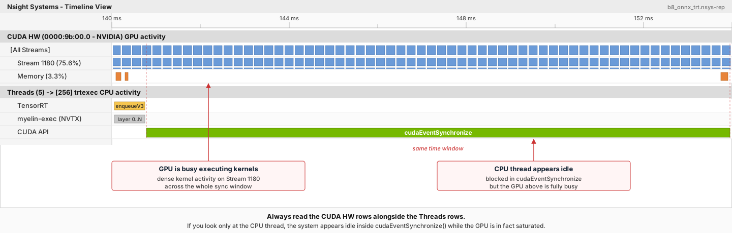
Figure 1 Reading the CUDA HW rows alongside the Threads rows in Nsight Systems. The long green cudaEventSynchronize band on the CUDA API row spans the same time window as the dense kernel activity on Stream 1180 above it: the CPU thread only appears idle while the GPU is in fact fully busy executing the enqueued work.#
The trtexec tool uses a slightly more complicated approach to enqueue the jobs: it enqueues the next query while the GPU is still executing the jobs from the previous query. For more information, refer to the trtexec section.
Use the NVTX Tracing in Nsight Systems
Tracing enables the NVIDIA Tools Extension SDK (NVTX), a C-based API for marking events and ranges in your applications. It allows Nsight Compute and Nsight Systems to collect data generated by TensorRT applications.
Decoding the kernel names back to layers in the original network can be complicated. Because of this, TensorRT uses NVTX to mark a range for each layer, allowing the CUDA profilers to correlate each layer with the kernels called to implement it. In TensorRT, NVTX helps to correlate the runtime engine layer execution with CUDA kernel calls. Nsight Systems supports collecting and visualizing these events and ranges on the timeline. Nsight Compute also supports collecting and displaying the state of all active NVTX domains and ranges in a given thread when the application is suspended.
In TensorRT, each layer can launch one or more kernels to perform its operations. The exact kernels launched depend on the optimized network and the hardware present. Depending on the builder’s choices, multiple additional operations that reorder data can be interspersed with layer computations; these reformat operations can be implemented as device-to-device memory copies or custom kernels.
On the Nsight Systems timeline, this appears as NVTX layer ranges on the CPU thread row aligned with the corresponding kernel ranges on the CUDA HW row underneath. Reformat copies show up as additional kernel ranges between layers, which makes them straightforward to spot when looking for unexpected overhead.
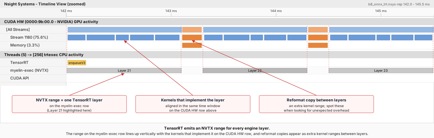
Figure 2 NVTX layer ranges on the myelin-exec row line up vertically with the kernel clusters that implement each layer on the CUDA HW row. Reformat copies between layers appear as additional (orange) kernel ranges - useful to spot when looking for unexpected overhead.#
Control the Level of Details in NVTX Tracing
By default, TensorRT only shows layer names in the NVTX markers. At the same time, users can control the level of details by setting the ProfilingVerbosity in the IBuilderConfig when the engine is built. For example, to disable NVTX tracing, set the ProfilingVerbosity to kNONE:
1builderConfig->setProfilingVerbosity(ProfilingVerbosity::kNONE);
1builder_config.profiling_verbosity = trt.ProfilingVerbosity.NONE
On the other hand, you can choose to allow TensorRT to print more detailed layer information in the NVTX markers, including input and output dimensions, operations, parameters, tactic numbers, and so on, by setting the ProfilingVerbosity to kDETAILED:
1builderConfig->setProfilingVerbosity(ProfilingVerbosity::kDETAILED);
1builder_config.profiling_verbosity = trt.ProfilingVerbosity.DETAILED
Note
Enabling detailed NVTX markers increases the latency of enqueueV3() calls and could result in a performance drop if the performance depends on the latency of enqueueV3() calls.
Run Nsight Systems with trtexec
Below is an example of the commands to gather Nsight Systems profiles using the trtexec tool:
trtexec --onnx=foo.onnx --profilingVerbosity=detailed --saveEngine=foo.plan
nsys profile -o foo_profile --capture-range cudaProfilerApi trtexec --profilingVerbosity=detailed --loadEngine=foo.plan --warmUp=0 --duration=0 --iterations=50
The first command builds and serializes the engine to foo.plan, and the second command runs the inference using foo.plan and generates a foo_profile.nsys-rep file that can then be opened in the Nsight Systems user interface for visualization.
The --profilingVerbosity=detailed flag allows TensorRT to show more detailed layer information in the NVTX marking, and the --warmUp=0, --duration=0, and --iterations=50 flags allow you to control how many inference iterations to run. By default, trtexec runs inference for three seconds, which can result in a large output of the nsys-rep file.
If the CUDA graph not disabled, add --cuda-graph-trace=node flag to the nsys command to view the per-kernel runtime information:
nsys profile -o foo_profile --capture-range cudaProfilerApi --cuda-graph-trace=node trtexec --profilingVerbosity=detailed --loadEngine=foo.plan --warmUp=0 --duration=0 --iterations=50
Optional: Enable GPU Metrics Sampling in Nsight Systems
On discrete GPU systems, add the --gpu-metrics-device all flag to the nsys command to sample GPU metrics, including GPU clock frequencies, DRAM bandwidth, and Tensor Core utilization. If the flag is added, these GPU metrics appear in the Nsight Systems web interface.
Profiling for DLA#
To profile DLA, add the --accelerator-trace nvmedia flag when using the NVIDIA Nsight Systems CLI or enable Collect other accelerators trace when using the user interface. For example, the following command can be used with the NVIDIA Nsight Systems CLI:
nsys profile -t cuda,nvtx,nvmedia,osrt --accelerator-trace=nvmedia --show-output=true trtexec --loadEngine=alexnet_int8.plan --warmUp=0 --duration=0 --iterations=20
Here is an example report:
NvMediaDLASubmitsubmits a DLA task for each DLA subgraph. The task’s runtime can be found in the DLA timeline under Other accelerators trace.Because GPU fallback was allowed, TensorRT automatically added some CUDA kernels, like
permutationKernelPLC3andcopyPackedKernel, which are used for data reformatting.EGLStreamAPIs were executed because TensorRT usesEGLStreamfor data transfer between GPU memory and DLA.
To maximize GPU utilization, trtexec enqueues the queries one batch beforehand. The runtime of the DLA task can be found under Other Accelerator API, alongside the CUDA kernels and EGLStream API calls used for interaction between the GPU and DLA.
Hardware/Software Environment for Performance Measurements#
A performance number is only as trustworthy as the environment it was collected in. Two runs of the same engine on the same GPU can disagree by tens of percent if the clock floats during one run and locks during the other, or if thermal throttling kicks in halfway through. This section catalogs the parts of the hardware and software environment that bias TensorRT measurements, what to watch for, and how to control or work around each one.
The subsections fall into three groups.
Stability of the GPU itself
GPU Information Query and GPU Monitoring - capture the baseline (
nvidia-smi -q) and a live trace (nvidia-smi dmon) of clocks, power, and temperature alongside every benchmark.GPU Clock Locking and Floating Clock - lock the clock for deterministic comparisons, let it float for peak performance.
GPU Power Consumption and Power Throttling - why power-capped GPUs (T4, A2) skew short-window throughput numbers.
GPU Temperature and Thermal Throttling - what happens at around 85 C, and how passive cooling and ambient airflow factor in.
Cost of moving data and launching work
H2D/D2H Data Transfers and PCIe Bandwidth - PCIe gen/lanes, pinned memory, NUMA placement, and the
--includeDataTransfersflag intrtexec.Enqueue-Bound Workloads and CUDA Graphs - when CPU launch overhead, not GPU compute, is the bottleneck, and how CUDA Graphs help.
Driver and synchronization configuration
GPU Driver Mode - on Windows, prefer TCC mode for dedicated inference GPUs.
BlockingSync and SpinWait Synchronization Modes - choose between more stable measurements (spin-wait) and lower CPU and power use (blocking-sync).
Important
The items involving nvidia-smi in this section are only supported on dGPU systems, not mobile platforms (Jetson, iGPU).
GPU Information Query and GPU Monitoring
While measuring performance, it is recommended that you record and monitor the GPU status in parallel to the inference workload. Having the monitoring data allows you to identify possible root causes when you encounter unexpected performance measurement results.
Before the inference starts, call the nvidia-smi -q command to get detailed information on the GPU, including the product name, power cap, clock settings. Then, while the inference workload is running, run the nvidia-smi dmon -s pcu -f <FILE> -c <COUNT> command in parallel to print out GPU clock frequencies, power consumption, temperature, and utilization to a file. Call nvidia-smi dmon --help for more options about the nvidia-smi device monitoring tool.
GPU Clock Locking and Floating Clock
By default, the GPU clock frequency is floating, meaning it sits idle when there is no active workload and boosts the boost clock frequency when the workload starts. This is usually the desired behavior since it allows the GPU to generate less heat at idle and to run at maximum speed when there is an active workload.
Alternatively, you can lock the clock at a specific frequency by calling the sudo nvidia-smi -lgc <freq> command (and conversely, you can let the clock float again with the sudo nvidia-smi -rgc command). The sudo nvidia-smi -q -d SUPPORTED_CLOCKS command can find the supported clock frequencies. After the clock frequency is locked, it should stay at that frequency unless power or thermal throttling occurs, which will be explained in the next sections. When the throttling kicks in, the device behaves like the clock floats.
Running TensorRT workloads with floating clocks or with throttling taking place can lead to more non-determinism in tactic selections and unstable performance measurements across inferences because every CUDA kernel can run at slightly different clock frequencies, depending on what frequency the driver boosts or throttles the clock to at that moment. On the other hand, running TensorRT workloads with locked clocks allows more deterministic tactic selections and consistent performance measurements. Still, the average performance will not be as good as when the clock is floating or is locked at maximum frequency with throttling taking place.
There is no definite recommendation on whether the clock should be locked or what clock frequency to lock the GPU while running TensorRT workloads. It depends on whether the deterministic and stable performance or the best average performance is desired.
GPU Power Consumption and Power Throttling
Power throttling occurs when the average GPU power consumption reaches the power limit, which can be set by the sudo nvidia-smi -pl <power_cap> command. When this happens, the driver has to throttle the clock to a lower frequency to keep the average power consumption below the limit. The constantly changing clock frequencies can lead to unstable performance measurements if the measurements are taken within a short time, such as within 20ms.
Power throttling happens by design and is a natural phenomenon when the GPU clock is not locked or is locked at a higher frequency, especially for GPUs with lower power limits, such as NVIDIA T4 and NVIDIA A2 GPUs. To avoid performance variations caused by power throttling, you can lock the GPU clock at a lower frequency to stabilize the performance numbers. However, the average performance numbers will be lower than those with floating clocks or the clock locked at a higher frequency, even though power throttling would happen in this case.
Another issue with power throttling is that it can skew the performance numbers if there are gaps between inferences in your performance benchmarking applications. For example, if the application synchronizes at each inference, there will be periods when the GPU is idle between the inferences. The gaps cause the GPU to consume less power on average, so the clock is throttled less, and the GPU can run at higher clock frequencies on average. However, the throughput numbers measured this way are inaccurate because when the GPU is fully loaded with no gaps between inferences, the actual clock frequency will be lower, and the actual throughput will not reach the throughput numbers measured using the benchmarking application.
To avoid this, the trtexec tool is designed to maximize GPU execution by leaving nearly no gaps between GPU kernel executions so that it can measure the true throughput of a TensorRT workload. Therefore, if you notice performance gaps between your benchmarking application and what trtexec reports, check if the power throttling and the gaps between inferences are the cause.
Lastly, power consumption can depend on the activation values, causing different input performance measurements. For example, if all the network input values are set to zeros or NaNs, the GPU consumes less power than when the inputs are normal values because of fewer bit-flips in DRAM and the L2 cache. To avoid this discrepancy, always use the input values that best represent the actual value distribution when measuring the performance. The trtexec tool uses random input values by default, but you can specify the input using the --loadInputs flag. For more information, refer to the trtexec section.
GPU Temperature and Thermal Throttling
Thermal throttling happens when the GPU temperature reaches a predefined threshold of around 85 degrees Celsius for most GPUs, and the driver has to throttle the clock to a lower frequency to prevent the GPU from overheating. You can tell this by seeing the temperature logged by the nvidia-smi dmon command gradually increasing while the inference workload runs until it reaches ~85C and the clock frequency drops.
If thermal throttling happens on actively cooled GPUs like the NVIDIA RTX A8000, then it is possible that the fans on the GPU are broken or obstacles are blocking the airflow.
If thermal throttling happens on passively cooled GPUs like NVIDIA A10, then it is likely that the GPUs are not properly cooled. Passively cooled GPUs require external fans or air conditioning to cool down the GPUs, and the airflow must go through the GPUs for effective cooling. Common cooling problems include installing GPUs in a server that is not designed for the GPUs or installing the wrong numbers of GPUs into the server. In some cases, the air flows through the “easy path” (the path with the least friction) around the GPUs instead of going through them. Fixing this requires examination of the airflow in the server and installation of airflow guidance if necessary.
Note that higher GPU temperature also leads to more leakage current in the circuits, which increases the power consumed by the GPU at a specific clock frequency. Therefore, for GPUs more likely to be power throttled like NVIDIA T4, poor cooling can lead to lower stabilized clock frequency with power throttling and, thus, worse performance, even if the GPU clocks have not been thermally throttled yet.
On the other hand, ambient temperature, the environment’s temperature around the server, does not usually affect GPU performance as long as the GPUs are properly cooled, except for GPUs with lower power limits whose performance can be slightly affected.
H2D/D2H Data Transfers and PCIe Bandwidth
On dGPU systems, the input data must often be copied from the host memory to the device memory (H2D) before an inference starts, and the output data must be copied back from the device memory to the host memory (D2H) after the inference. These H2D/D2H data transfers go through PCIe buses, and they can sometimes influence the inference performance or even become the performance bottleneck. The H2D/D2H copies can also be seen in the Nsight Systems profiles, appearing as cudaMemcpy() or cudaMemcpyAsync() CUDA API calls.
To achieve maximum throughput, the H2D/D2H data transfers should run parallel to the GPU executions of other inferences so that the GPU does not sit idle when the H2D/D2H copies occur. This can be done by running multiple inferences in parallel streams or launching H2D/D2H copies in a different stream than the stream used for GPU executions and using CUDA events to synchronize between the streams. The trtexec tool shows an example of the latter implementation.
When the H2D/D2H copies run parallel to GPU executions, they can interfere with the GPU executions, especially if the host memory is pageable, which is the default case. Therefore, it is recommended that you allocate pinned host memory for the input and output data using cudaHostAlloc() or cudaMallocHost() CUDA APIs.
To check whether the PCIe bandwidth becomes the performance bottleneck, you can check the Nsight Systems profiles to determine whether the H2D or D2H copies of an inference query have longer latencies than the GPU execution part. If PCIe bandwidth becomes the performance bottleneck, here are a few possible solutions.
First, check whether the PCIe bus configuration of the GPU is correct in terms of what generation (such as Gen3 or Gen4) and how many lanes (such as x8 or x16) are used. Next, reduce the amount of data that must be transferred using the PCIe bus. For example, suppose the input images have high resolutions, and the H2D copies become the bottleneck. In that case, you can transmit JPEG-compressed images over the PCIe bus and decode the image on the GPUs before the inference workflow instead of transmitting raw pixels. Finally, consider using NVIDIA GPUDirect technology to load data directly from/to the network or the filesystems without going through the host memory.
In addition, if your system has AMD x86_64 CPUs, check the machine’s NUMA (Non-Uniform Memory Access) configurations with the numactl --hardware command. The PCIe bandwidth between a host memory and a device memory located on two different NUMA nodes is much more limited than the bandwidth between the host/device memory located on the same NUMA node. Allocate the host memory on the NUMA node on which the GPU that will receive the copied data resides. Also, pin the CPU threads that trigger the H2D/D2H copies on that specific NUMA node.
Note that the host and the device share the same memory on mobile platforms, so the H2D/D2H data transfers are not required if the host memory is allocated using CUDA APIs and is pinned instead of pageable.
By default, the trtexec tool excludes the latencies of the H2D/D2H data transfers. You can add the --includeDataTransfers flag to include the latencies of the H2D/D2H data transfers to see if the H2D/D2H copies can bottleneck the TensorRT workload.
GPU Driver Mode
On Windows, configure the GPU to TCC (Tesla Compute Cluster) mode for best inference performance:
nvidia-smi -dm 1
In TCC mode, the GPU focuses on computation work, and graphics support like OpenGL or monitor display is disabled. This is the recommended mode for GPUs that run TensorRT inference workloads.
Warning
A GPU connected to a display must not be configured into TCC mode.
For more information, refer to the TCC mode documentation.
WDDM (Windows Display Driver Model) mode supports both graphics and compute but tends to cause GPUs to have worse and unstable performance results when running inference workloads using TensorRT. Use TCC mode when possible for dedicated inference GPUs.
Linux does not have a TCC/WDDM mode distinction. The GPU driver is always in compute-capable mode. No driver mode configuration is needed for TensorRT inference on Linux.
Enqueue-Bound Workloads and CUDA Graphs
The enqueueV3() function of IExecutionContext is asynchronous. That is, it returns immediately after all the CUDA kernels are launched without waiting for the completion of CUDA kernel executions. However, in some cases, the enqueueV3() time can take longer than the actual GPU executions, causing the latency of enqueueV3() calls to become the performance bottleneck. We say that this type of workload is “enqueue-bound.” Two reasons can cause a workload to be enqueue-bound.
First, if the workload is very tiny in terms of the number of computations, such as containing convolutions with small I/O sizes, matrix multiplications with small GEMM sizes, or mostly element-wise operations throughout the network, then the workload tends to be enqueue-bound. This is because most CUDA kernels take the CPU and the driver around 5-15 microseconds to launch per kernel, so if each CUDA kernel execution time is only several microseconds long on average, the kernel launching time becomes the main performance bottleneck.
To solve this, try increasing the computation per CUDA kernel by increasing the batch size. You can also use CUDA Graphs to capture the kernel launches into a graph and launch the graph instead of calling enqueueV3().
Second, it is naturally queue-bound if the workload contains operations requiring device synchronizations, such as loops or if-else conditions. Increasing the batch size can help improve the throughput without increasing the latency.
In trtexec, CUDA graphs are enabled by default. You can add the --noCudaGraph flag to disable the use of CUDA graphs and check if a workload is enqueue-bound by checking whether the reported Enqueue Time is close to or longer than the reported GPU Compute Time.
BlockingSync and SpinWait Synchronization Modes
If performance is measured with cudaStreamSynchronize() or cudaEventSynchronize(), synchronization overhead variations can lead to performance measurement variations. This section describes the causes of the variations and how to avoid them.
When cudaStreamSynchronize() is called, there are two ways in which the driver waits until the stream is completed. If the cudaDeviceScheduleBlockingSync flag has been set with cudaSetDeviceFlags() calls, then the cudaStreamSynchronize() uses the blocking-sync mechanism. Otherwise, it uses the spin-wait mechanism.
A similar idea applies to CUDA events. If a CUDA event is created with the cudaEventDefault flag, then the cudaEventSynchronize() call uses the spin-wait mechanism. If a CUDA event is created with the cudaEventBlockingSync flag, then the cudaEventSynchronize() call will use the blocking-sync mechanism.
When the blocking-sync mode is used, the host thread yields to another thread until the device work is done. This allows the CPUs to sit idle to save power or to be used by other CPU workloads when the device is still executing. However, the blocking-sync mode tends to result in relatively unstable overheads in stream/event synchronizations in some OS, leading to variations in latency measurements.
On the other hand, when the spin-wait mode is used, the host thread is constantly polling until the device work is done. Using spin-wait makes the latency measurements more stable due to shorter and more stable overhead in stream/event synchronizations. Still, it consumes some CPU computation resources and leads to more power consumption by the CPUs.
Therefore, if you want to reduce CPU power consumption or do not want the stream/event synchronizations to consume CPU resources (such as you are running other heavy CPU workloads in parallel), use the blocking-sync mode. If you care more about stable performance measurements, use the spin-wait mode.
In trtexec, the default synchronization mechanism is in spin-wait mode. You can add the --blockingSync flag to enable synchronizations using the blocking-sync mode for less CPU utilizations and less power consumption at the cost of more unstable latency measurements.