Pre-Deployment Profiling#
Tip
New to SLA Planner? For a complete workflow including profiling and deployment, see the SLA Planner Quick Start Guide.
Profiling Script#
To ensure Dynamo deployments comply with the SLA, we provide a pre-deployment script to profile the model performance with different parallelization mappings and recommend the parallelization mapping for prefill and decode workers and planner configurations. To use this script, the user needs to provide the target ISL, OSL, TTFT SLA, and ITL SLA.
Note
Time Investment: This profiling process is comprehensive and typically takes a few hours to complete. The script systematically tests multiple tensor parallelism configurations and load conditions to find optimal performance settings. This upfront investment ensures your deployment meets SLA requirements and operates efficiently.
Support matrix:
Backends |
Model Types |
Supported |
|---|---|---|
vLLM |
Dense |
✅ |
vLLM |
MoE |
🚧 |
SGLang |
Dense |
✅ |
SGLang |
MoE |
✅ |
TensorRT-LLM |
Dense |
✅ |
TensorRT-LLM |
MoE |
🚧 |
Note
The script considers a fixed ISL/OSL without KV cache reuse. If the real ISL/OSL has a large variance or a significant amount of KV cache can be reused, the result might be inaccurate.
We assume there is no piggy-backed prefill requests in the decode engine. Even if there are some short piggy-backed prefill requests in the decode engine, it should not affect the ITL too much in most conditions. However, if the piggy-backed prefill requests are too much, the ITL might be inaccurate.
The script will first detect the number of available GPUs on the current nodes (multi-node engine not supported yet). Then, it will profile the prefill and decode performance with different TP sizes. For prefill, since there is no in-flight batching (assume isl is long enough to saturate the GPU), the script directly measures the TTFT for a request with given isl without kv-reusing. For decode, since the ITL (or iteration time) is relevant with how many requests are in-flight, the script will measure the ITL under different number of in-flight requests. The range of the number of in-flight requests is from 1 to the maximum number of requests that the kv cache of the engine can hold. To measure the ITL without being affected by piggy-backed prefill requests, the script will enable kv-reuse and warm up the engine by issuing the same prompts before measuring the ITL. Since the kv cache is sufficient for all the requests, it can hold the kv cache of the pre-computed prompts and skip the prefill phase when measuring the ITL.
GPU Resource Usage#
Important: Profiling tests different tensor parallelism (TP) configurations sequentially, not in parallel. This means:
One TP configuration at a time: Each tensor parallelism size (TP1, TP2, TP4, TP8, etc.) is tested individually
Full GPU access: Each TP configuration gets exclusive access to all available GPUs during its profiling run
Resource isolation: No interference between different TP configurations during testing
Accurate measurements: Each configuration is profiled under identical resource conditions
This sequential approach ensures:
Precise performance profiling without resource conflicts
Consistent GPU allocation for fair comparison across TP sizes
Reliable cleanup between different TP configuration tests
Accurate SLA compliance verification for each configuration
After the profiling finishes, two plots will be generated in the output-dir. For example, here are the profiling results for components/backends/vllm/deploy/disagg.yaml:
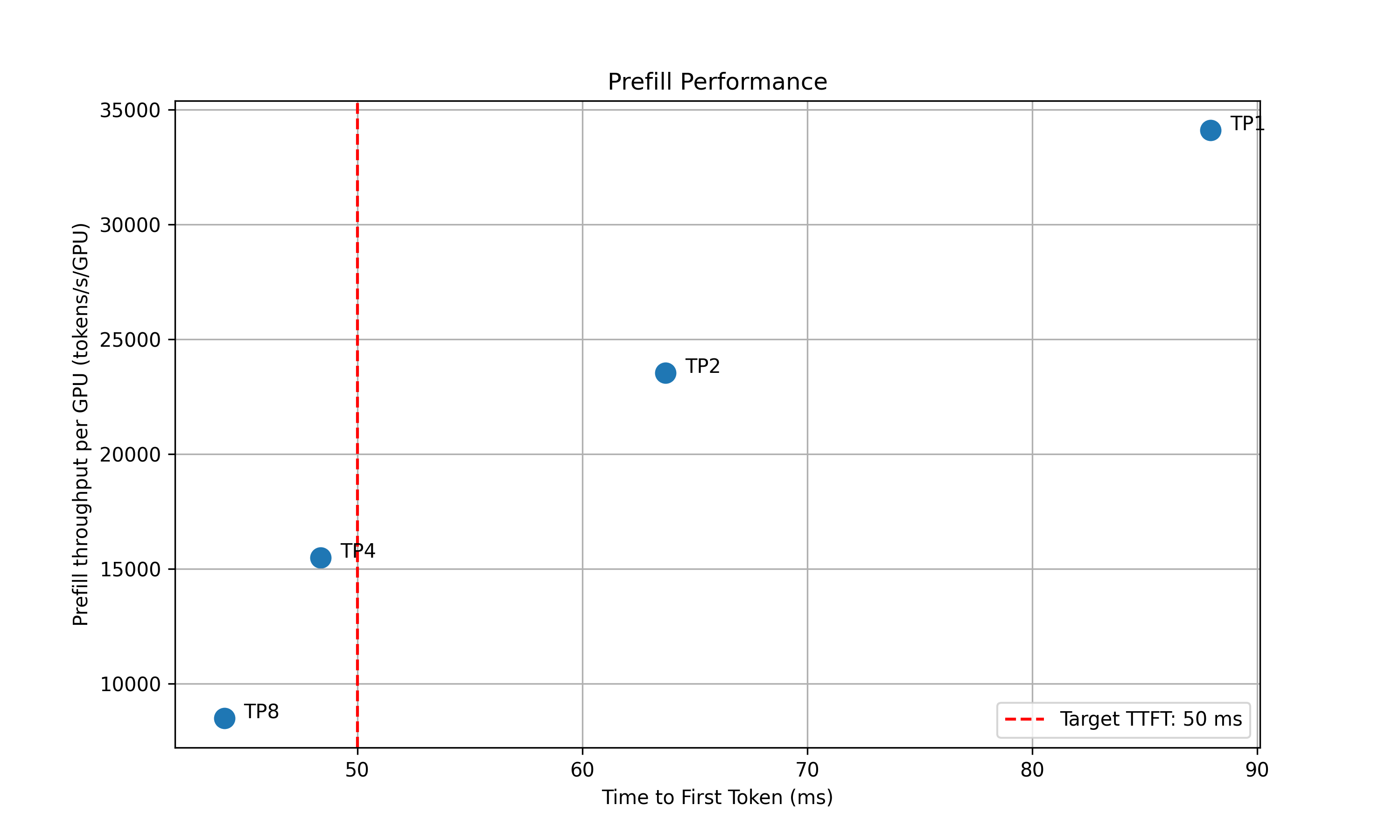
For the prefill performance, the script will plot the TTFT for different TP sizes and select the best TP size that meet the target TTFT SLA and delivers the best throughput per GPU. Based on how close the TTFT of the selected TP size is to the SLA, the script will also recommend the upper and lower bounds of the prefill queue size to be used in planner.
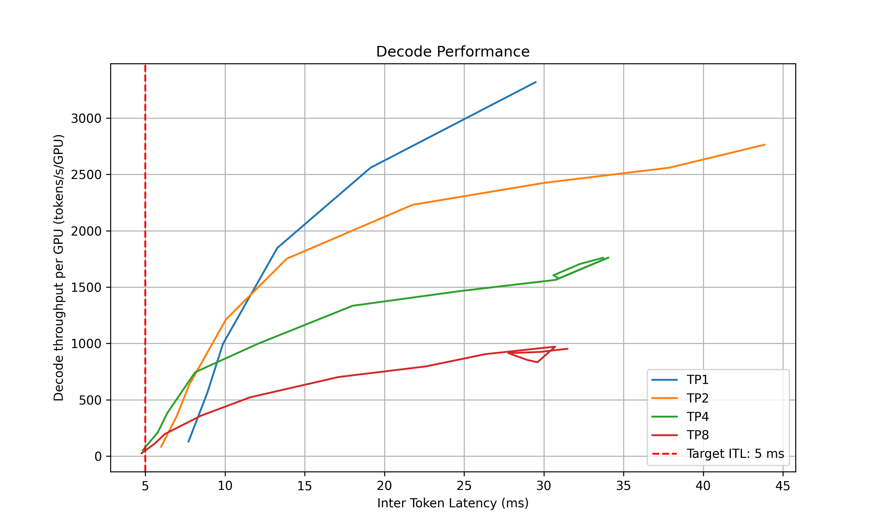
For the decode performance, the script will plot the ITL for different TP sizes and different in-flight requests. Similarly, it will select the best point that satisfies the ITL SLA and delivers the best throughput per GPU and recommend the upper and lower bounds of the kv cache utilization rate to be used in planner.
The script will recommend the best TP size for prefill and decode, as well as the upper and lower bounds of the prefill queue size and decode kv cache utilization rate if using load-based planner. The following information will be printed out in the terminal:
2025-05-16 15:20:24 - __main__ - INFO - Analyzing results and generate recommendations...
2025-05-16 15:20:24 - __main__ - INFO - Suggested prefill TP:4 (TTFT 48.37 ms, throughput 15505.23 tokens/s/GPU)
2025-05-16 15:20:24 - __main__ - INFO - Suggested planner upper/lower bound for prefill queue size: 0.24/0.10
2025-05-16 15:20:24 - __main__ - INFO - Suggested decode TP:4 (ITL 4.83 ms, throughput 51.22 tokens/s/GPU)
2025-05-16 15:20:24 - __main__ - INFO - Suggested planner upper/lower bound for decode kv cache utilization: 0.20/0.10
After finding the best TP size for prefill and decode, the script will then interpolate the TTFT with ISL and ITL with active KV cache and decode context length. This is to provide a more accurate estimation of the performance when ISL and OSL changes and will be used in the sla-planner. The results will be saved to <output_dir>/<decode/prefill>_tp<best_tp>_interpolation. Please change the prefill and decode TP size in the config file to match the best TP sizes obtained from the profiling script.
Prefill Interpolation Data#
In prefill engine, prefills are usually done with batch size=1 and only the ISL (excluding prefix cache hit) affects the iteration time. The script profiles the selected prefill TP configuration across different ISLs and record the TTFT and prefill throughput per GPU under those ISLs.
For dense models, the script profiles different TP sizes. For MoE models, the script only profiles different TEP sizes, since DEP is generally not the optimal prefill configuration.
Decode Interpolation Data#
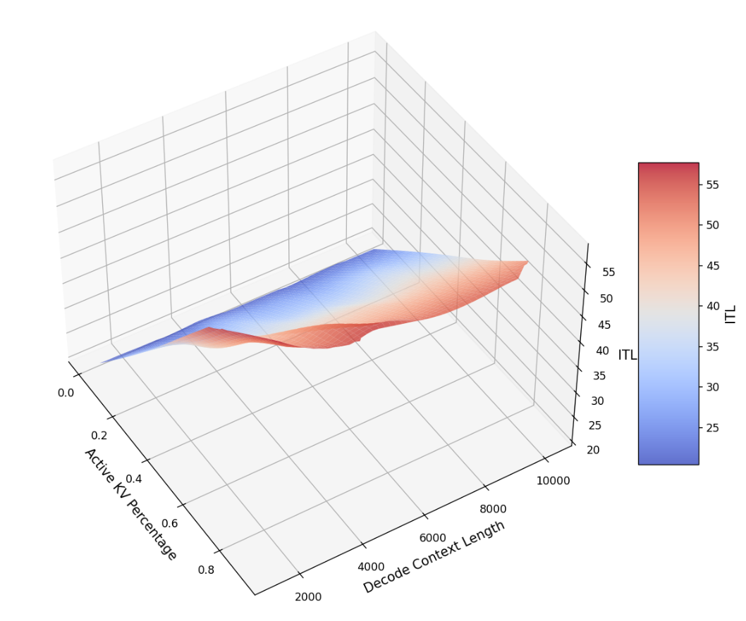
In decode engine, decode requests are added inflight and iteration time (or ITL) depends on both the context length and the real-time load of the engine. We capture the real-time load of the engine with active kv usage and average context length. The active kv usage determines the complexity of the memory-bounded attention kernel while the active kv usage divided the average context length determines the complexity of the computation bound MLP kernel. For example, the below figure shows the ITL of DS-Distilled Llama 8b model on H100 TP4. The ITL grows near-linearly with active kv usage under a fixed context length. And the slope increases as the context length decreases.
For dense models, the script profiles different TP sizes. For MoE models, the script profiles different DEP sizes. TEP decode engines for low latency will be supported in the future.
The script profiles the selected decode TP configuration across different active kv blocks and average context length.
Output Format of Interpolation Data#
After suggesting the optimal TP configuration, two .npz files that describe the performance characteristics of the prefill and decode engines in their suggested parallel configurations will be generated. The two .npz files are:
${benchmark_result_dir}/selected_prefill_interpolation/raw_data.npz}prefill_isl: a 1D Numpy array to store the ISLs used to profile the prefill engine.prefill_ttft: a 1D Numpy array to store the TTFTs under the corresponding ISLs when the prefill engine is exclusively running each prefill request (i.e., with batch size of 1). The unit is in milliseconds.prefill_thpt_per_gpu: a 1D Numpy array to store the prefill throughput per GPU under the corresponding ISLs. The unit is in tokens per second per GPU.
${benchmark_result_dir}/selected_decode_interpolation/raw_data.npzmax_kv_tokens: a 1D Numpy array with only one element to store the total number of KV tokens in the decode engine.x_kv_usage: a 1D Numpy array to store the percentage of the active KV blocks (in the range of [0, 1]) used to profile the decode engine. The active KV blocks can be controlled by varying(ISL + OSL / 2) * concurrency.y_context_length: a 1D Numpy array to store the average context length (ISL + OSL / 2) used to profile the decode engine.z_itl: a 1D Numpy array to store the ITLs under the corresponding active KV usage and context length. To skip the prefill stage while maintaining the context length, benchmark can be done by turn on kv reuse and warmup the engine with the prompts first before running the actual profiling. The unit is in milliseconds.z_thpt_per_gpu: a 1D Numpy array to store the decode throughput per GPU under the corresponding active KV usage and context length. The unit is in tokens per second per GPU.
SLA planner can work with any interpolation data that follows the above format. For best results, use fine-grained and high coverage interpolation data for the prefill and decode engines.
Detailed Kubernetes Profiling Instructions#
Tip
For a complete step-by-step workflow, see the SLA Planner Quick Start Guide.
This section provides detailed technical information for advanced users who need to customize the profiling process.
Configuration Options#
For dense models, configure $DYNAMO_HOME/benchmarks/profiler/deploy/profile_sla_job.yaml:
spec:
  template:
    spec:
      containers:
        - name: profile-sla
          args:
            - --isl
            - "3000" # average ISL is 3000 tokens
            - --osl
            - "150" # average OSL is 150 tokens
            - --ttft
            - "200" # target TTFT is 200ms (float, in milliseconds)
            - --itl
            - "20" # target ITL is 20ms (float, in milliseconds)
            - --backend
            - <vllm/sglang>
For MoE models, use profile_sla_moe_job.yaml with TEP/DEP configuration instead.
If you want to automatically deploy the optimized DGD with planner after profiling, add --deploy-after-profile to the profiling job. It will deploy the DGD with the engine of the optimized parallelization mapping found for the SLA targets.
Advanced Configuration#
Model caching: For large models, create a multi-attach PVC to cache the model. See recipes for details.
Custom disaggregated configurations: Use the manifest injector to place custom DGD configurations in the PVC.
Planner Config Passthrough: To specify custom planner configurations (e.g.,
adjustment-intervalorload-predictor) in the generated or deployed DGD config, add aplanner-prefix to the argument. For example, to specify--adjustment-interval=60in SLA planner, add--planner-adjustment-interval=60arg to the profiling job.Resource allocation: Modify the job YAML to adjust GPU and memory requirements.
Viewing Profiling Results#
After the profiling job completes successfully, the results are stored in the persistent volume claim (PVC) created during Step 2.
To download the results:
# Download to directory
python3 -m deploy.utils.download_pvc_results --namespace $NAMESPACE --output-dir ./results --folder /data/profiling_results

# Download without any of the auto-created config.yaml files used in profiling
python3 -m deploy.utils.download_pvc_results --namespace $NAMESPACE --output-dir ./results --folder /data/profiling_results --no-config
The script will:
Deploy a temporary access pod
Download all files maintaining directory structure
Clean the pod up automatically
File Structure#
The profiling results directory contains the following structure:
/workspace/data/profiling_results/
├── prefill_performance.png                    # Main prefill performance plot
├── decode_performance.png                     # Main decode performance plot
├── prefill_tp1/                               # Individual TP profiling directories
...
├── decode_tp1/
...
├── selected_prefill_interpolation/
│   ├── raw_data.npz                           # Prefill interpolation data
│   ├── prefill_ttft_interpolation.png         # TTFT vs ISL plot
│   └── prefill_throughput_interpolation.png   # Throughput vs ISL plot
├── selected_decode_interpolation/
│   ├── raw_data.npz                           # Decode interpolation data
│   └── decode_tp{best_tp}.png                 # 3D ITL surface plot
└── config_with_planner.yaml                   # Generated DGD config with planner
Viewing Performance Plots#
The profiling generates several performance visualization files:
Main Performance Plots:
prefill_performance.png: Shows TTFT (Time To First Token) performance across different tensor parallelism (TP) sizesdecode_performance.png: Shows ITL (Inter-Token Latency) performance across different TP sizes and in-flight request counts
Interpolation Plots:
selected_prefill_interpolation/prefill_ttft_interpolation.png: TTFT vs Input Sequence Length with quadratic fitselected_prefill_interpolation/prefill_throughput_interpolation.png: Prefill throughput vs Input Sequence Lengthselected_decode_interpolation/decode_tp{best_tp}.png: 3D surface plot showing ITL vs KV usage and context length
Understanding the Data Files#
The .npz files contain raw profiling data that can be loaded and analyzed using Python:
import numpy as np

# Load prefill data
prefill_data = np.load('selected_prefill_interpolation/raw_data.npz')
print("Prefill data keys:", list(prefill_data.keys()))

# Load decode data
decode_data = np.load('selected_decode_interpolation/raw_data.npz')
print("Decode data keys:", list(decode_data.keys()))
Troubleshooting#
Image Pull Authentication Errors#
If you see ErrImagePull or ImagePullBackOff errors with 401 unauthorized messages:
Ensure the
nvcr-imagepullsecretexists in your namespace:kubectl get secret nvcr-imagepullsecret -n $NAMESPACE
Verify the service account was created with the image pull secret:
kubectl get serviceaccount dynamo-sa -n $NAMESPACE -o yaml
The service account should show
imagePullSecretscontainingnvcr-imagepullsecret.
If it doesn’t, create the secret
export NGC_API_KEY=<you-ngc-api-key-here>
kubectl create secret docker-registry nvcr-imagepullsecret --docker-server=nvcr.io --docker-username='$oauthtoken' --docker-password=$NGC_API_KEY
Running the Profiling Script with AI Configurator#
Note
TensorRT-LLM Only: AI Configurator currently supports TensorRT-LLM only. Support for vLLM and SGLang is coming soon.
The profiling script can be run much faster using AI Configurator to estimate performance numbers instead of running real Dynamo deployments. This completes profiling in 20-30 seconds using performance simulation.
Advantages of --use-ai-configurator:
Script completes in seconds rather than hours
No Kubernetes or GPU access required
Ideal for rapid prototyping and testing
Disadvantages:
Estimated performance may contain errors, especially for out-of-distribution input dimensions
Limited list of supported models, systems, and backends
Less accurate than real deployment profiling
Prerequisites#
Install AI Configurator:
pip install aiconfigurator
If using local environment, also install:
pip install -r deploy/utils/requirements.txt
Check Support Matrix#
View supported models, systems, and backends:
aiconfigurator cli --help
Supported configurations:
Models: GPT_7B, GPT_13B, GPT_30B, GPT_66B, GPT_175B, LLAMA2_7B, LLAMA2_13B, LLAMA2_70B, LLAMA3.1_8B, LLAMA3.1_70B, LLAMA3.1_405B, MOE_Mixtral8x7B, MOE_Mixtral8x22B, DEEPSEEK_V3, KIMI_K2, QWEN2.5_1.5B, QWEN2.5_7B, QWEN2.5_32B, QWEN2.5_72B, QWEN3_32B, QWEN3_235B, QWEN3_480B, Nemotron_super_v1.1

Systems: h100_sxm, h200_sxm

Backends: trtllm (vllm and sglang support coming soon)
Running Fast Profiling#
Example command for TensorRT-LLM:
python3 -m benchmarks.profiler.profile_sla \
   --config ./components/backends/trtllm/deploy/disagg.yaml \
   --backend trtllm \
   --use-ai-configurator \
   --aic-system h200_sxm \
   --aic-model-name QWEN3_32B \
   --aic-backend trtllm \ # optional, will use --backend if not provided
   --aic-backend-version 0.20.0 \
   --isl 3000 \
   --osl 150 \
   --ttft 200 \ # target TTFT in milliseconds (float)
   --itl 20 # target ITL in milliseconds (float)
The output will be written to ./profiling_results/ and can be used directly with SLA planner deployment.