Darcy Flow with Physics-Informed Fourier Neural Operator

Introduction

This tutorial solves the 2D Darcy flow problem using Physics-Informed Neural Operators (PINO) [1]. In this tutorial, you will learn:

1. Differences between PINO and Fourier Neural Operators (FNO).

2. How to set up and train PINO in PhysicsNeMo Sym.

3. How to define a custom PDE constraint for grid data.

Note

This tutorial assumes that you are familiar with the basic functionality of PhysicsNeMo Sym and understand the PINO architecture. Please see the Introductory Example and Physics Informed Neural Operator sections for additional information. Additionally, this tutorial builds upon the Darcy Flow with Fourier Neural Operator which should be read prior to this one.

Warning

The Python package gdown is required for this example if you do not already have the example data downloaded and converted. Install using pip install gdown.

Problem Description

This problem illustrates developing a surrogate model that learns the mapping between a permeability and pressure field of a Darcy flow system. The mapping learned, \(\textbf{K} \rightarrow \textbf{U}\), should be true for a distribution of permeability fields \(\textbf{K} \sim p(\textbf{K})\) and not just a single solution.

The key difference between PINO and FNO is that PINO adds a physics-informed term to the loss function of FNO. As discussed further in the Physics Informed Neural Operator theory, the PINO loss function is described by:

\[\mathcal{L} = \mathcal{L}_{data} + \mathcal{L}_{pde},\]

where

\[\mathcal{L}_{data} = \lVert u - \mathcal{G}_\theta(a) \rVert^2 ,\]

where \(\mathcal{G}_\theta(a)\) is a FNO model with learnable parameters \(\theta\) and input field \(a\), and \(\mathcal{L}_{pde}\) is an appropriate PDE loss. For the 2D Darcy problem (see Darcy Flow with Fourier Neural Operator) this is given by

\[\mathcal{L}_{pde} = \lVert -\nabla \cdot \left(k(\textbf{x})\nabla \mathcal{G}_\theta(a)(\textbf{x})\right) - f(\textbf{x}) \rVert^2 ,\]

where \(k(\textbf{x})\) is the permeability field, \(f(\textbf{x})\) is the forcing function equal to 1 in this case, and \(a=k\) in this case.

Note that the PDE loss involves computing various partial derivatives of the FNO ansatz, \(\mathcal{G}_\theta(a)\). In general this is nontrivial; in PhysicsNeMo Sym, three different methods for computing these are provided. These are based on the original PINO paper:

1. Numerical differentiation computed via finite difference Method (FDM)

2. Numerical differentiation computed via spectral derivative

3. Numerical differentiation based on the “exact” Fourier / automatic differentiation approach [2]

Note that the last approach only works for a fixed decoder model. Upon enabling “exact” gradient calculations, the decoder network will switch to a 2 layer fully-connected model with Tanh activations. This is because this approach requires an expensive Hessian calculation. The Hessian calculation is explicitly defined for this two layer model, thus avoiding automatic differentiation which would be otherwise be extremely expensive.

Case setup

The setup for this problem is largely the same as the FNO example (Darcy Flow with Fourier Neural Operator), except that the PDE loss is defined and the FNO model is constrained using it. This process is described in detail in Defining PDE Loss below.

Similar to the FNO chapter, the training and validation data for this example can be found on the Fourier Neural Operator Github page. However, an automated script for downloading and converting this dataset has been included. This requires the package gdown which can easily installed through pip install gdown.

Note

The python script for this problem can be found at examples/darcy/darcy_pino.py.

Configuration

The configuration for this problem is similar to the FNO example, but importantly there is an extra parameter custom.gradient_method where the method for computing the gradients in the PDE loss is selected. This can be one of fdm, fourier, exact corresponding to the three options above. The balance between the data and PDE terms in the loss function can also be controlled using the loss.weights parameter group.

# SPDX-FileCopyrightText: Copyright (c) 2023 - 2024 NVIDIA CORPORATION & AFFILIATES.
# SPDX-FileCopyrightText: All rights reserved.
# SPDX-License-Identifier: Apache-2.0
#
# Licensed under the Apache License, Version 2.0 (the "License");
# you may not use this file except in compliance with the License.
# You may obtain a copy of the License at
#
#     http://www.apache.org/licenses/LICENSE-2.0
#
# Unless required by applicable law or agreed to in writing, software
# distributed under the License is distributed on an "AS IS" BASIS,
# WITHOUT WARRANTIES OR CONDITIONS OF ANY KIND, either express or implied.
# See the License for the specific language governing permissions and
# limitations under the License.

defaults :
  - physicsnemo_default
  - /arch/conv_fully_connected_cfg@arch.decoder
  - /arch/fno_cfg@arch.fno
  - scheduler: tf_exponential_lr
  - optimizer: adam
  - loss: sum
  - _self_

cuda_graphs: false
jit: false

custom:
  gradient_method: exact
  ntrain: 1000
  ntest: 100

arch:
  decoder:
    input_keys: [z, 32]
    output_keys: sol
    nr_layers: 1
    layer_size: 32

  fno:
    input_keys: coeff
    dimension: 2
    nr_fno_layers: 4
    fno_modes: 12
    padding: 9

scheduler:
  decay_rate: 0.95
  decay_steps: 1000

training:
  rec_results_freq : 1000
  max_steps : 10000

loss:
  weights:
    sol: 1.0
    darcy: 0.1

batch_size:
  grid: 8
  validation: 8

Defining PDE Loss

For this example, a custom PDE residual calculation is defined using the various approaches proposed above. Defining a custom PDE residual using sympy and automatic differentiation is discussed in 1D Wave Equation, but in this problem you will not be relying on standard automatic differentiation for calculating the derivatives. Rather, you will explicitly define how the residual is calculated using a custom torch.nn.Module called Darcy. The purpose of this module is to compute and return the Darcy PDE residual given the input and output tensors of the FNO model, which is done via its .forward(...) method:

from physicsnemo.models.layers import fourier_derivatives # helper function for computing spectral derivatives
from ops import dx, ddx # helper function for computing finite difference derivatives

class Darcy(torch.nn.Module):
    "Custom Darcy PDE definition for PINO"

    def __init__(self, gradient_method: str = "exact"):
        super().__init__()
        self.gradient_method = str(gradient_method)

    def forward(self, input_var: Dict[str, torch.Tensor]) -> Dict[str, torch.Tensor]:
        # get inputs
        u = input_var["sol"]
        c = input_var["coeff"]
        dcdx = input_var["Kcoeff_y"]  # data is reversed
        dcdy = input_var["Kcoeff_x"]

        dxf = 1.0 / u.shape[-2]
        dyf = 1.0 / u.shape[-1]
        # Compute gradients based on method
        # Exact first order and FDM second order
        if self.gradient_method == "exact":
            dudx_exact = input_var["sol__x"]
            dudy_exact = input_var["sol__y"]
            dduddx_exact = input_var["sol__x__x"]
            dduddy_exact = input_var["sol__y__y"]
            # compute darcy equation
            darcy = (
                1.0
                + (dcdx * dudx_exact)
                + (c * dduddx_exact)
                + (dcdy * dudy_exact)
                + (c * dduddy_exact)
            )
        # FDM gradients
        elif self.gradient_method == "fdm":
            dudx_fdm = dx(u, dx=dxf, channel=0, dim=0, order=1, padding="replication")
            dudy_fdm = dx(u, dx=dyf, channel=0, dim=1, order=1, padding="replication")
            dduddx_fdm = ddx(
                u, dx=dxf, channel=0, dim=0, order=1, padding="replication"
            )
            dduddy_fdm = ddx(
                u, dx=dyf, channel=0, dim=1, order=1, padding="replication"
            )
            # compute darcy equation
            darcy = (
                1.0
                + (dcdx * dudx_fdm)
                + (c * dduddx_fdm)
                + (dcdy * dudy_fdm)
                + (c * dduddy_fdm)
            )
        # Fourier derivative
        elif self.gradient_method == "fourier":
            dim_u_x = u.shape[2]
            dim_u_y = u.shape[3]
            u = F.pad(
                u, (0, dim_u_y - 1, 0, dim_u_x - 1), mode="reflect"
            )  # Constant seems to give best results
            f_du, f_ddu = fourier_derivatives(u, [2.0, 2.0])
            dudx_fourier = f_du[:, 0:1, :dim_u_x, :dim_u_y]
            dudy_fourier = f_du[:, 1:2, :dim_u_x, :dim_u_y]
            dduddx_fourier = f_ddu[:, 0:1, :dim_u_x, :dim_u_y]
            dduddy_fourier = f_ddu[:, 1:2, :dim_u_x, :dim_u_y]
            # compute darcy equation
            darcy = (
                1.0
                + (dcdx * dudx_fourier)
                + (c * dduddx_fourier)
                + (dcdy * dudy_fourier)
                + (c * dduddy_fourier)
            )
        else:
            raise ValueError(f"Derivative method {self.gradient_method} not supported.")

        # Zero outer boundary
        darcy = F.pad(darcy[:, :, 2:-2, 2:-2], [2, 2, 2, 2], "constant", 0)
        # Return darcy
        output_var = {
            "darcy": dxf * darcy,
        }  # weight boundary loss higher
        return output_var

The gradients of the FNO solution are computed according to the gradient method selected above. The FNO model automatically outputs first and second order gradients when the exact method is used, and so no extra computation of these is necessary. Furthermore, note that the gradients of the permeability field are already included as tensors in the FNO input training data (with keys Kcoeff_x and Kcoeff_y) and so these do not need to be computed.

Next, incorporate this module into PhysicsNeMo Sym by wrapping it into a PhysicsNeMo Sym Node. This ensures the module is incorporated into PhysicsNeMo Sym’ computational graph and can be used to optimise the FNO.

from physicsnemo.sym.node import Node

    # Make custom Darcy residual node for PINO
    inputs = [
        "sol",
        "coeff",
        "Kcoeff_x",
        "Kcoeff_y",
    ]
    if cfg.custom.gradient_method == "exact":
        inputs += [
            "sol__x",
            "sol__y",
        ]
    darcy_node = Node(
        inputs=inputs,
        outputs=["darcy"],
        evaluate=Darcy(gradient_method=cfg.custom.gradient_method),
        name="Darcy Node",
    )
    nodes = [fno.make_node("fno"), darcy_node]

Finally, define the PDE loss term by adding a constraint to the darcy output variable (see Adding Constraints below).

Loading Data

Loading both the training and validation datasets follows a similar process as the FNO example:

    # load training/ test data
    input_keys = [
        Key("coeff", scale=(7.48360e00, 4.49996e00)),
        Key("Kcoeff_x"),
        Key("Kcoeff_y"),
    ]
    output_keys = [
        Key("sol", scale=(5.74634e-03, 3.88433e-03)),
    ]

    download_FNO_dataset("Darcy_241", outdir="datasets/")
    invar_train, outvar_train = load_FNO_dataset(
        "datasets/Darcy_241/piececonst_r241_N1024_smooth1.hdf5",
        [k.name for k in input_keys],
        [k.name for k in output_keys],
        n_examples=cfg.custom.ntrain,
    )
    invar_test, outvar_test = load_FNO_dataset(
        "datasets/Darcy_241/piececonst_r241_N1024_smooth2.hdf5",
        [k.name for k in input_keys],
        [k.name for k in output_keys],
        n_examples=cfg.custom.ntest,
    )

    # add additional constraining values for darcy variable
    outvar_train["darcy"] = np.zeros_like(outvar_train["sol"])

    train_dataset = DictGridDataset(invar_train, outvar_train)
    test_dataset = DictGridDataset(invar_test, outvar_test)

Initializing the Model

Initializing the model also follows a similar process as the FNO example:

    # Define FNO model
    decoder_net = instantiate_arch(
        cfg=cfg.arch.decoder,
        output_keys=output_keys,
    )
    fno = instantiate_arch(
        cfg=cfg.arch.fno,
        input_keys=[input_keys[0]],
        decoder_net=decoder_net,
    )
    if cfg.custom.gradient_method == "exact":
        derivatives = [
            Key("sol", derivatives=[Key("x")]),
            Key("sol", derivatives=[Key("y")]),
            Key("sol", derivatives=[Key("x"), Key("x")]),
            Key("sol", derivatives=[Key("y"), Key("y")]),
        ]
        fno.add_pino_gradients(
            derivatives=derivatives,
            domain_length=[1.0, 1.0],
        )

However, in the case where the exact gradient method is used, you need to additionally instruct the model to output the appropriate gradients by specifying these gradients in its output keys.

Adding Constraints

Finally, add constraints to your model in a similar fashion to the FNO example. The same SupervisedGridConstraint can be used; to include the PDE loss term you need to define additional target values for the darcy output variable defined above (zeros, to minimise the PDE residual) and add them to the outvar_train dictionary:

    # make domain
    domain = Domain()

    # add constraints to domain
    supervised = SupervisedGridConstraint(
        nodes=nodes,
        dataset=train_dataset,
        batch_size=cfg.batch_size.grid,
    )
    domain.add_constraint(supervised, "supervised")

The same data validator as the FNO example is used.

Training the Model

The training can now be simply started by executing the python script.

python darcy_PINO.py

Results and Post-processing

The checkpoint directory is saved based on the results recording frequency specified in the rec_results_freq parameter of its derivatives. See Results Frequency for more information. The network directory folder (in this case 'outputs/darcy_pino/validators') contains several plots of different validation predictions.

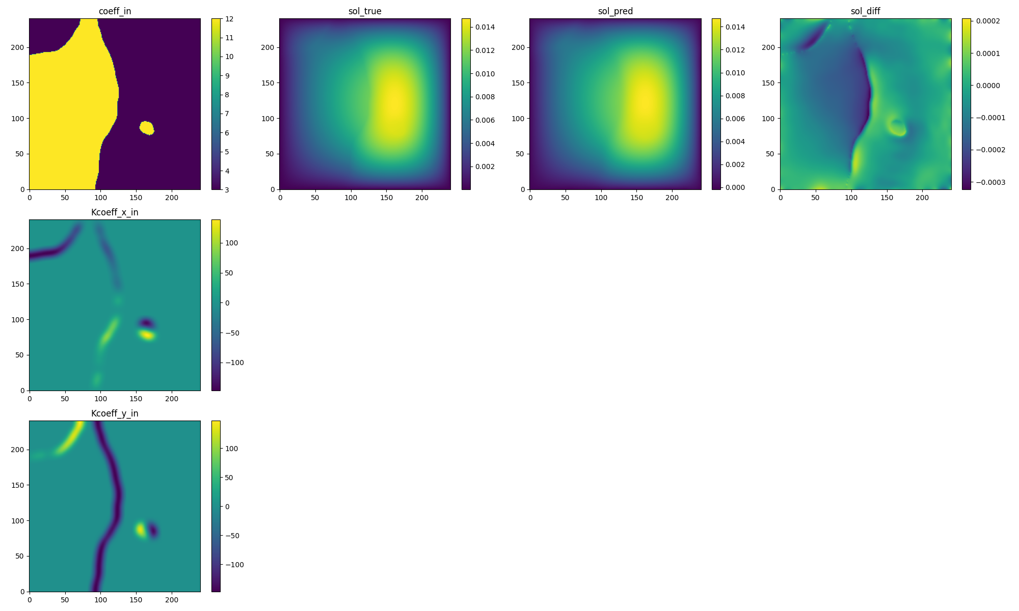
Fig. 123 PINO validation prediction. (Left to right) Input permeability and its spatial derivatives, true pressure, predicted pressure, error.

Comparison to FNO

The TensorBoard plot below compares the validation loss of PINO (all three gradient methods) and FNO. You can see that with large amounts of training data (1000 training examples), both FNO and PINO perform similarly.

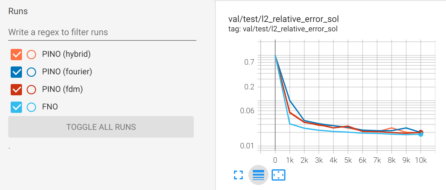
Fig. 124 Comparison between PINO and FNO accuracy for surrogate modeling Darcy flow.

A benefit of PINO is that the PDE loss regularizes the model, meaning that it can be more effective in “small data” regimes. The plot below shows the validation loss when both models are trained with only 100 training examples:

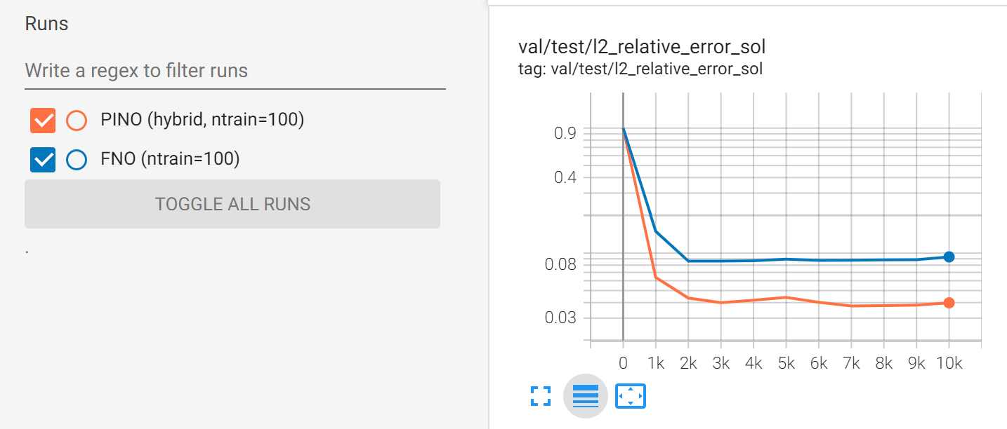
Fig. 125 Comparison between PINO and FNO accuracy for surrogate modeling Darcy flow (small data regime).

You can observe that, in this case, the PINO outperforms the FNO.

References / Footnotes

[1]

Li, Zongyi, et al. “Physics-informed neural operator for learning partial differential equations.” arXiv preprint arXiv:2111.03794 (2021).

[2]

Note that the “exact” method is technically not exact because it uses a combination of numerical spectral derivatives and exact differentiation. See the original paper for more details.