Recommended Practices in PhysicsNeMo Sym#

Physics Informed Neural Networks#

Some of the improvements like adding integral continuity planes, weighting the losses spatially, and varying the point density in the areas of interest, have been key in making PhysicsNeMo Sym robust and capable of handling some of the larger scale problems. In this section we will dive into details for some of the important ones.

Scaling and Nondimensionalizing the Problem#

The input geometry of the problem can be scaled such that the characteristic length is closer to unity and the geometry is centered around origin. Also, it is often advantageous to work with the nondimensionalized form of physical quantities and PDEs. This can be achieved by output scaling, or nondimensionalizing the PDEs itself using some characteristic dimensions and properties. Simple tricks like these can help improve the convergence behavior and can also give more accurate results. More information on nondimensionalizing the PDEs can be found in Scaling of Differential Equations. Several examples in the User Guide already adopt this philosophy. Some examples where such nondimensionalizing is extensively leveraged are: Linear Elasticity, Heat Transfer with High Thermal Conductivity, Industrial Heat Sink, etc.

PhysicsNeMo Sym provides some utilities based on the Pint python library to facilitate scaling and nondimensionalization. With this, the user can define a quantity in PhysicsNeMo Sym which represents a physical quantity with a value and a unit. Pint has a powerful string parsing support and the specified units do not necessarily have to follow a strict format. For example, the velocity unit can be defined as meter/second, m/s, or meter/s. Different algebraic manipulations can be done on different PhysicsNeMo Sym quantities and PhysicsNeMo Sym will automatically keep track of the units. The user can instantiate a nondimensionalizer object by providing the required characteristics scales to the NonDimensionalizer method, and this object can be used to scale and nondimensionalize the quantities.

An example using scaling and nondimensionalization with Pint based utilities is located in examples/cylinder/cylinder_2d.py for learning the flow around a cylinder. A Scaler node is used for scaling back the nondimensionalized quantities to any target quantity with user specified units for post-processing purposes and for inference or validation domains.

Integral Continuity Planes#

For some of the fluid flow problems involving channel flow, we found that, in addition to solving the Navier-Stokes equations in differential form, specifying the mass flow through some of the planes in the domain significantly speeds up the rate of convergence and gives better accuracy. Assuming there is no leakage of flow, we can guarantee that the flow exiting the system must be equal to the flow entering the system. Also, we found that by specifying such constraints at several other planes in the interior improves the accuracy further. For incompressible flows, one can replace mass flow with the volumetric flow rate.

Fig. 55 shows the comparison of adding more integral continuity planes and points in the interior, applied to a problem of solving flow over a 3D 3-fin heat sink in a channel (tutorial Parameterized 3D Heat Sink). The one IC plane case has just one IC plane at the outlet while the 11 IC plane case has 10 IC planes in the interior in addition to the IC plane at the outlet. A lower mass imbalance inside the system indicates that the case run with 11 integral continuity planes helps in satisfying the continuity equation better and faster.

Fig. 55 Improvements in accuracy by adding more Integral continuity planes and points inside the domain#

Spatial Weighting of Losses (SDF weighting)#

One area of considerable interest is weighting the losses with respect to each other. For example, we can weight the losses from equation (1) in the following way,

\[L = \lambda_{BC}L_{BC} + \lambda_{residual}L_{residual}\]

Depending on the \(\lambda_{BC}\) and \(\lambda_{residual}\) this can impact the convergence of the solver. We can extend this idea to varying the weightings spatially as well. Written out in the integral formulation of the losses we get,

\[L_{residual} = \int_0^1 \lambda_{residual}(x) \left( \frac{\delta^2 u_{net}}{\delta x^2}(x) - f(x) \right)^2 dx\]

The choice for the \(\lambda_{residual}(x)\), can be varied based on problem definition, and is an active field of research. In general, we have found it beneficial to weight losses lower on sharp gradients or discontinuous areas of the domain. For example, if there are discontinuities in the boundary conditions we may have the loss decay to \(0\) on these discontinuities. Another example is weighting the equation residuals by the signed distance function, SDF, of the geometries. If the geometry has sharp corners this often results in sharp gradients in the solution of the differential equation. Weighting by the SDF tends to weight these sharp gradients lower and often results in a convergence speed increase and sometimes also improved accuracy. In this user guide there are many examples of this and we defer further discussion to the specific examples.

Fig. 56 shows \(L_2\) errors for one such example of laminar flow (Reynolds number 50) over a 17 fin heat sink (tutorial FPGA Heat Sink with Laminar Flow) in the initial 100,000 iterations. The multiple closely spaced thin fins lead to several sharp gradients in flow equation residuals in the vicinity of the heat sink. Weighting them spatially, we essentially minimize the dominance of these sharp gradients during the iterations and achieve a faster rate of convergence.

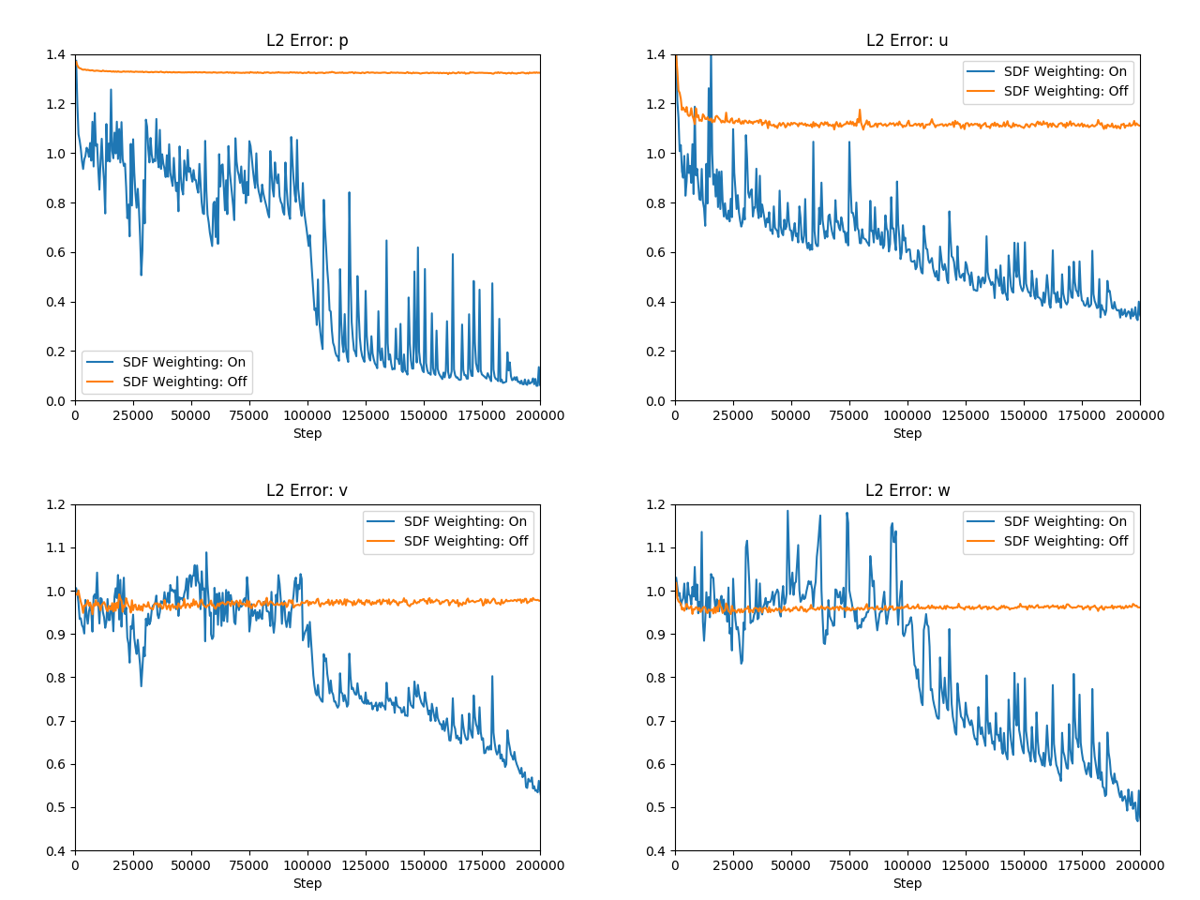
Fig. 56 Improvements in convergence speed by weighting the equation residuals spatially.#

A similar weighting is also applied to the intersection of boundaries where there are discontinuities. We will cover this in detail in the first tutorial on the Lid Driven Cavity flow (tutorial Introductory Example).

Increasing the Point Cloud Density#

In this section, we discuss the accuracy improvements by adding more points in the areas where the field is expected to show a stronger spatial variation. This is somewhat similar to the FEM/FVM approach where the mesh density is increased in the areas where we wish to resolve the field better. If too few points are used when training then an issue can occur where the network may be satisfying the equation and boundary conditions correctly on these points but not in the spaces between these points. Quantifying the required density of points needed is an open research question however in practice if the validation losses or the validation residuals losses start to increase towards the end of training then more points may be necessary.

Fig. 57 shows the comparison of increasing the point density in the vicinity of the same 17 fin heat sink that we saw in the earlier comparison in Section Spatial Weighting of Losses (SDF weighting), but now with a Reynolds number of 500 and with zero equation turbulence. Using more points near the heat sink, we are able to achieve better \(L_2\) errors for \(p\), \(v\), and \(w\).

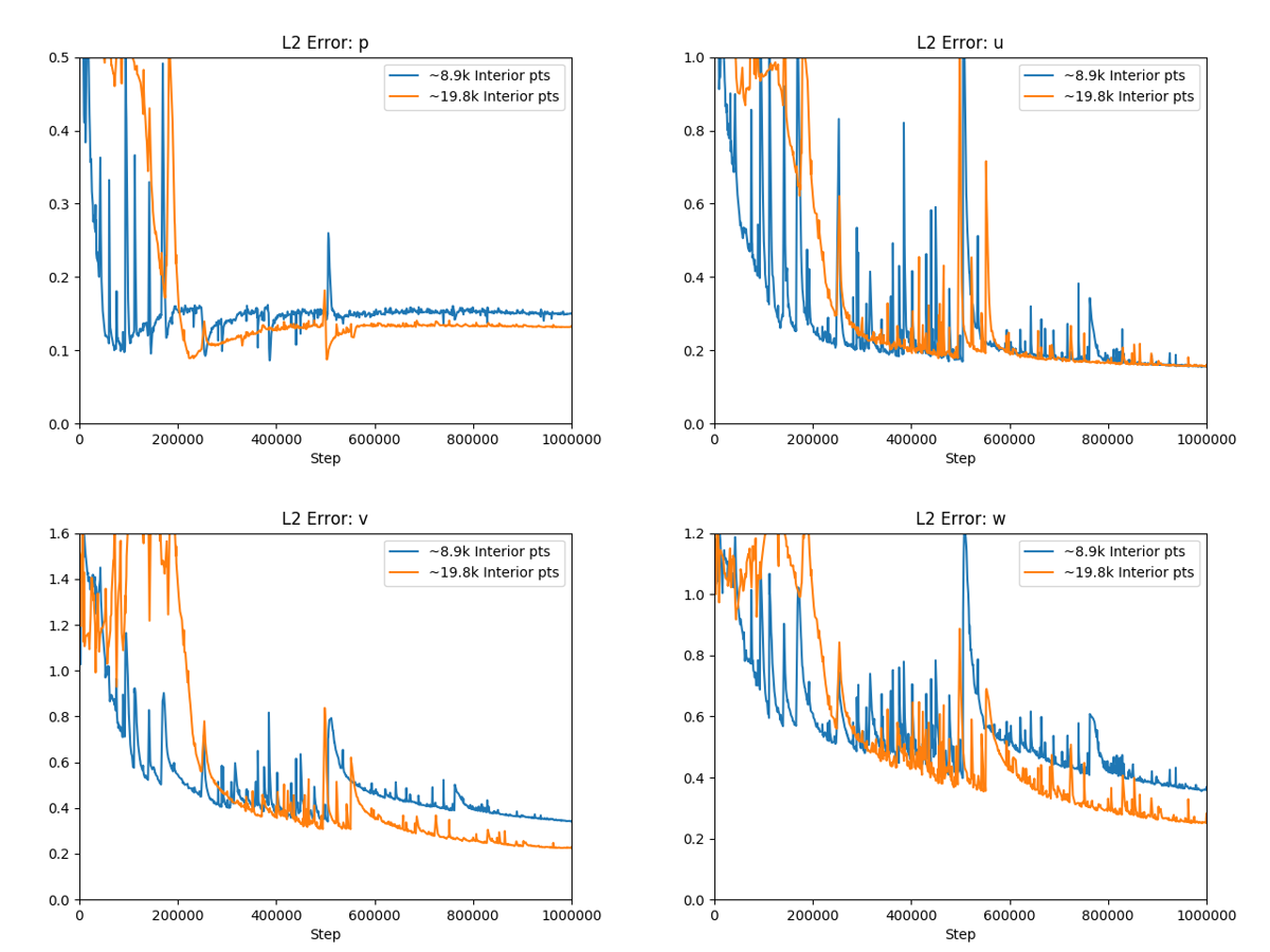
Fig. 57 Improvements in accuracy by adding more points in the interior.#

Note

Care should be taken while increasing the integral continuity planes and adding more points in the domain as one might run into memory issues while training. If one runs into such an issue, some ways to avoid that would be to reduce the points sampled during each batch and increasing the number of GPUs. Another way is to use gradient aggregation, which is discussed next.

Gradient Aggregation#

As mentioned in the previous subsection, training of a neural network solver for complex problems requires a large batch size that can be beyond the available GPU memory limits. Increasing the number of GPUs can effectively increase the batch size, however, one can instead use gradient aggregation in case of limited GPU availability. With gradient aggregation, the required gradients are computed in several forward/backward iterations using different mini batches of the point cloud and are then aggregated and applied to update the model parameters. This will, in effect, increase the batch size, although at the cost of increasing the training time. In the case of multi-GPU/node training, gradients corresponding to each mini-batch are aggregated locally on each GPU, and are then aggregated globally just before the model parameters are updated. Therefore, gradient aggregation does not introduce any extra communication overhead between the workers. Details on how to use the gradient aggregation in PhysicsNeMo Sym is provided in Tutorial PhysicsNeMo Sym Configuration.

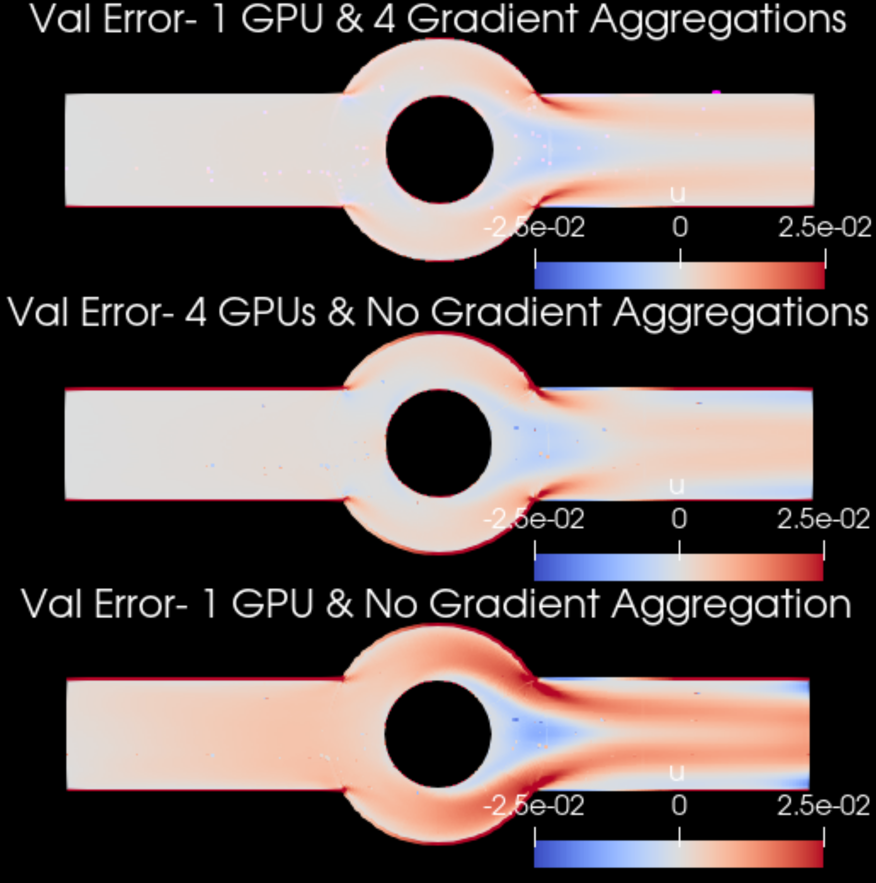
Increasing the batch size can improve the accuracy of neural network solvers. Results are for the :math:`u`-velocity of an annular ring example trained with different number of GPUs and gradient aggregations. — Fig. 58 Increasing the batch size can improve the accuracy of neural network solvers. Results are for the \(u\)-velocity of an annular ring example trained with different number of GPUs and gradient aggregations.#

Exact Continuity#

Velocity-pressure formulations are the most widely used formulations of the Navier-Stokes equation. However, this formulation has two issues that can be challenging to deal with. The first is the pressure boundary conditions, which are not given naturally. The second is the absence of pressure in the continuity equation, in addition to the fact that there is no evolution equation for pressure that may allow to adjust mass conservation. A way to ensure mass conservation is the definition of the velocity field from a vector potential:

\[\vec{V}=\nabla \times \vec{\psi}=\left(\frac{\partial \psi_{z}}{\partial y}-\frac{\partial \psi_{y}}{\partial z}, \frac{\partial \psi_{x}}{\partial z}-\frac{\partial \psi_{z}}{\partial x}, \frac{\partial \psi_{y}}{\partial x}-\frac{\partial \psi_{x}}{\partial y}\right)^{T},\]

where \(\vec{\psi}=\left(\psi_{x}, \psi_{y}, \psi_{z}\right)\). This definition of the velocity field ensures that it is divergence free and that it satisfies continuity:

\[\nabla \cdot \vec{V}=\nabla \cdot(\nabla \times \vec{\psi})=0.\]

A good overview of related formulations and their advantages can be found in [1].

Symmetry#

In training of PINNs for problems with symmetry in geometry and physical quantities, reducing the computational domain and using the symmetry boundaries can help with accelerating the training, reducing the memory usage, and in some cases, improving the accuracy. In PhysicsNeMo Sym, the following symmetry boundary conditions at the line or plane of symmetry may be used:

Zero value for the physical variables with odd symmetry.
Zero normal gradient for physical variables with even symmetry.

Details on how to setup an example with symmetry boundary conditions are presented in tutorial FPGA Heat Sink with Laminar Flow.

Operator Learning Networks#

In this subsection, we provide some recommendations about operator learning networks. Literally, operator learning networks is aiming to learn operators or parametrized operators between two function spaces. There are two networks structures now in PhysicsNeMo Sym that can handle this problem, DeepONet and Fourier Neural Operator. Both of these two structures have data informed and physics informed modeling ways.

For data informed approach, the computational graph is relative simply as there is no gradients involved in the loss terms. However, you must provide enough data to train. This can be obtained by numerical solvers or real experiments. For physics informed approach, there is no need of data for training, but only a few data for validation. Instead, physical laws are used to train the network. So the computational graph is relatively large, and need more time to train. You may choose your own structure depending on the problem.

DeepONet#

The Deep operator network (DeepONet) consist of branch net and trunk net. The branch net takes features from the input functions, while the trunk net takes features from the final evaluation points. If the input function data is defined on a grid, then some special network structure can be used in branch net, such as CNN or Fourier neural operator. We found these structures are more efficient than fully-connected because they can extract feature from the data more efficiently.

The trunk net will decide where we evaluate the output functions. Therefore, we may select a suitable network structure for the trunk net. For example, if the output function is of high frequency, we may use Fourier networks with a suitable frequency. This will make the network much easier to train.

For the concrete examples of DeepONet in PhysicsNeMo Sym, please see tutorial DeepONet.

References