Graphical User Interface#

The important elements in the graphical user interface are outlined in the following figure:

interface

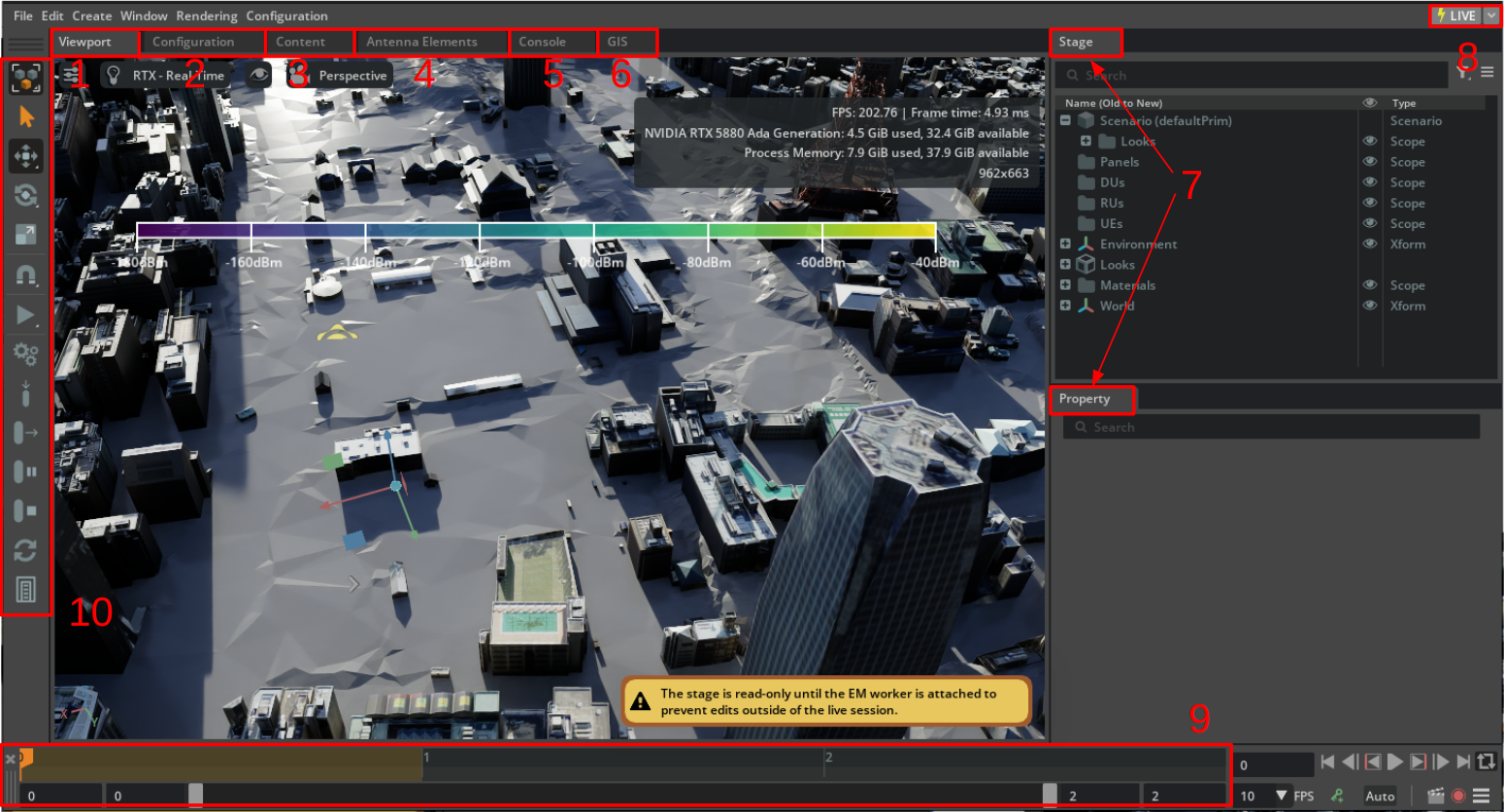
1. Viewport tab#

The viewport displays the geospatial data that makes up the scenario and is used to deploy the radio access network (RAN) nodes or specific user equipment (UE). At the top of the viewport, you can also find the settings to change the view type (e.g. top or perspective) or viewport resolution. Finally, the color bar provides a gradient that describes the power carried by each individual ray traced by the EM engine; it can be hidden or shown using CTRL+B.

Context Menu#

The viewport context menu, accessible with a right-click, provides several deployment options for radio access network (RAN) components.

Right-clicking on the map reveals the following deployment options under the Aerial submenu:

Deploy RU (Radio Unit): Deploys a radio unit at the selected location, which transmits and receives radio signals to/from user equipment.
Deploy DU (Distributed Unit): Deploys a distributed unit that serves as the processing hub for associated radio units, handling baseband processing.
Deploy UE (User Equipment): Manually deploys user equipment (mobile devices) at the selected location for precise positioning and testing purposes.
Deploy Spawn Zone: Creates a designated area where procedural user equipment can be automatically generated during large-scale simulations.

Under the Map Tools submenu, you can find the following:

Copy Coordinates: Copies the latitude/longitude coordinates of the mouse click location to the clipboard.
Place Pin: Places a pin at the specified location, either by latitude/longitude or mouse click. The color is configurable.
Update Georeferencing: Adds or changes scene georeferencing. First, select a known landmark. Then, input its latitude/longitude coordinates and EPSG code. You must use a projected coordinate system.
Validate Map: Checks the opened map for common errors. This is especially useful when the map is created outside of AODT.
Visualize Roads: Adds a primitive representing the road network. You must select a map.osm file for the map, which is typically located in the map assets folder. This feature is particularly useful for urban mobility.
Additional Options: Enables experimental features.

Configuration tab#

The configuration tab is used to set up the simulation and offers the following fields:

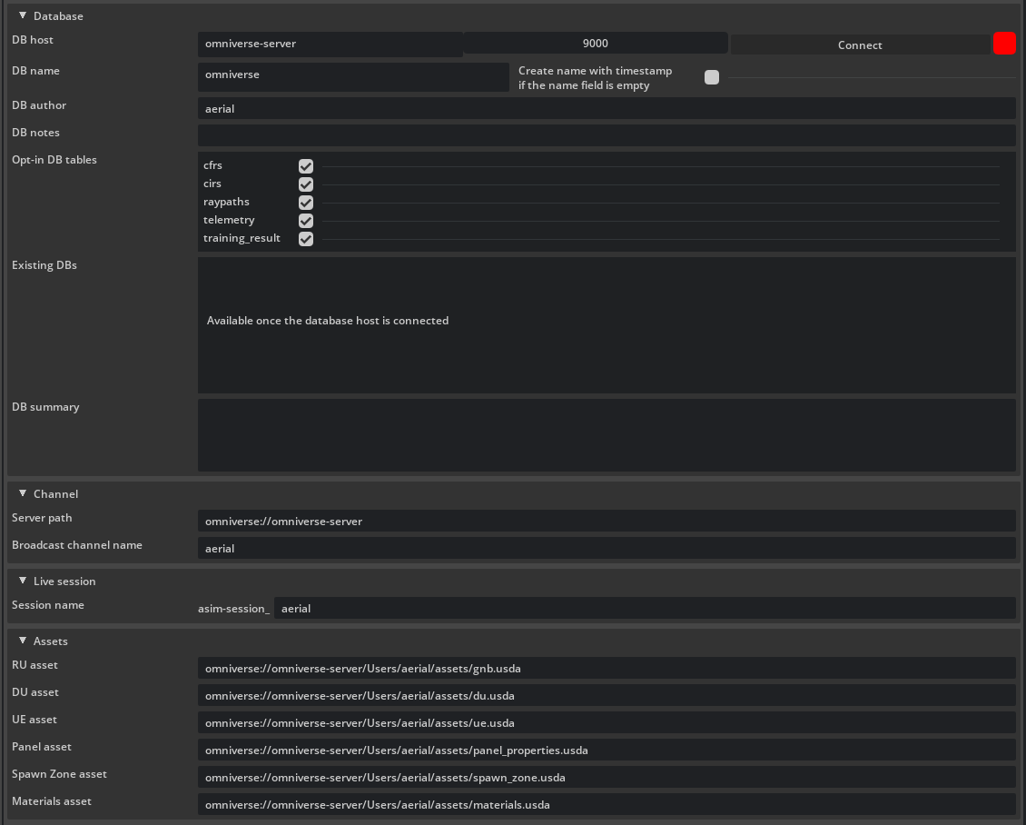
Database
- DB host: Specifies the IP address of the ClickHouse server.
- DB port: Indicates the ClickHouse client port. By default, this field is 9000, unless ClickHouse has been installed with non-standard settings. Once the DB host and DB port are specified, the user can connect to the ClickHouse server using the Connect button. If the connection is successful, the indicator next to the button will go from red to green.
- DB name: This is the name of the database that will be used to store the results generated during the simulation.
- DB author: This field records the author of the database. By default, it is the user ID.
- DB notes: This field includes any additional text that the user intends to add to the database. This field can be left empty.
- Opt-in DB tables: This list contains output tables that can be opted in or out for storing simulation results. The default behavior is to opt in.
- Existing DBs: Displays a list of databases available on the DB host once connected. Starting from release 1.2, databases containing simulation results can be displayed on the UI by clicking the Replay button on the corresponding entry or by double-clicking on the entry itself.
- DB summary: the summary of the DB selected from Existing DBs, also available once the host is connected.
NATS Message Broker
- NATS server path: the URL of the NATS server to connect to. This can be a local server (e.g., localhost) or a remote one, depending on your deployment. Ensure that workers also have network access and credentials to access the server (if required).
- NATS message subject: the subject of the NATS message that the workers and the UI will listen to. Subjects act like lightweight topics in NATS and are used to route messages.
Assets
- Session name: the name of the Omniverse live session used by the UI and the workers.
- RU asset: the URL to the 3D asset used to indicate a radio unit.
- DU asset: the URL to the 3D asset used to indicate a distributed unit.
- UE asset: the URL to the 3D asset used to indicate a UE.
- Materials asset: the URL pointing to the asset that describes the ITU P.2040 materials used within the scope of the simulation.
- Vehicle Scatterer asset: the URL to the 3D asset used to indicate a vehicular dynamic scatterer (car).

3. Content tab#

The content tab can be used to browse the content of the Nucleus server, move/copy files, and open the desired scene. Changes made in the live session will always be stored in a directory adjacent to the USD file, within a .live directory. To reset the scene to its initial state, delete the .live directory located in the same folder as the scene.

4. Console tab#

This tab is used to illustrate all warnings and messages collected during the operation of the Aerial Omniverse Digital Twin. Warnings are marked in yellow, and errors are marked in red. Errors of consequence for the simulation are also propagated to a dialog box.

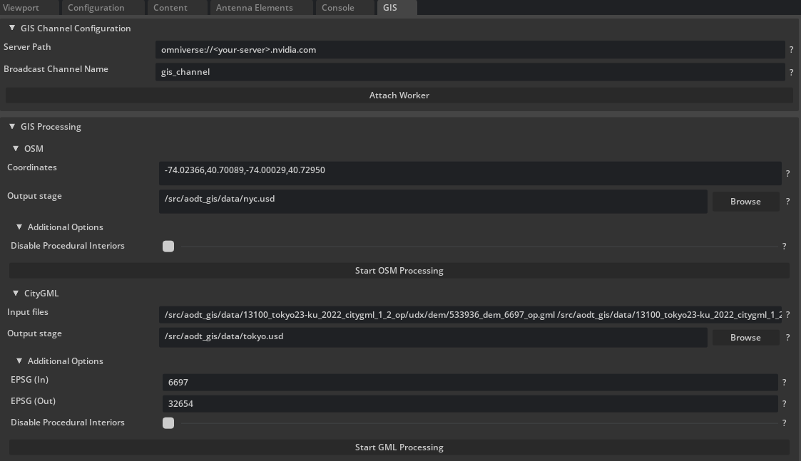
5. GIS tab#

The GIS tab is used to connect to the GIS container and trigger USD conversion jobs from CityGML or OpenStreetMap (OSM) sources. It offers the following fields:

NATS Message Broker
- NATS server path: the URL of the NATS server to connect to. This can be a local server (e.g., localhost) or a remote one, depending on your deployment. Ensure that the worker has network access and the necessary credentials (if required) to connect to the server.
- NATS message subject: the subject of the NATS message that the worker and UI will listen to. Subjects act like lightweight topics in NATS and are used to route messages.
GIS Processing:
- OSM: contains configuration for OSM processing.
  - Coordinates: coordinates for the bounding box used for OSM import. Must be in decimal degrees and in the following order: lower-left longitude, lower-left latitude, upper-right longitude, upper-right latitude.
  - Output stage: URL of the output USD stage.
  - Additional Options:
    - Disable Procedural Interiors: specifies whether the GIS pipeline should avoid generating procedural indoor spaces for the imported buildings.
- CityGML: contains configuration for CityGML processing.
  - Input files: a list of CityGML paths on the host of the GIS container.
  - Output stage: URL of the output USD stage
  - Additional Options:
    - EPSG (In): EPSG code of incoming CityGML data
    - EPSG (Out): EPSG code of resulting USD stage. Must be a projected coordinate system (linear units).
    - Disable Procedural Interiors: specifies whether the GIS pipeline should avoid generating procedural indoor spaces for the imported buildings.

6. Antenna Elements tab#

The antenna tab is used while setting up the simulation to specify

the type of antennas that a given antenna panel is composed of
the geometrical and polarimetric properties of such a panel.

The fields of the tab are illustrated in the following figure.

antenna_elements

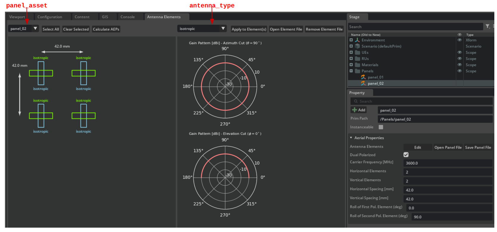
After visually selecting one or more antenna elements in the array, the Antenna Type combo box edits their antenna type. In particular,
- the user can select the antenna elements whose antenna type needs to be changed by clicking on the elements in the simplified diagram of the array, where the element using the first linear polarization are marked in blue and those using the second polarization are represented in green
- the user can then select the antenna type from the Antenna Type combo box,
- and finally apply it using the Apply to Element(s) button.

If successful, the type of the antenna element is updated in the diagram. To add or remove a second polarization, update the Dual Polarized check box in the property widget.

Below are the supported built-in antenna types:

isotropic
polarized isotropic
infinitesimal dipole
halfwave dipole
microstrip patch, with
- \(\epsilon_r=4.8\)
- \(L = \dfrac{\lambda}{2 \sqrt{\epsilon_r}}\) (\(\lambda\) being the wavelength of the carrier)
- \(W = 1.5 L\)
3GPP-type for radio unit element

while custom antenna elements can be imported using the button

Open Element File, which supports a single element CSV or FFD file upload. The file needs to have the section header [Antenna element parameters] and the pattern data for a single antenna element with header columns Theta,Phi,EThetaReal,EThetaImag,EPhiReal,EPhiImag. Once a pattern file is uploaded, the pattern will be added to the Antenna Type combo box and can be applied to the selected elements. The patterns can be removed using the Remove Element File button. Any antenna element for which its pattern is removed will revert back isotropic.

For halfwave dipoles, the Aerial Omniverse Digital Twin also offers the possibility of directly calculating the active antenna element pattern (AEP) for each element with the button Calculate AEP, thus accounting for mutual coupling effects.

In the tab we also find two plots:

the gain pattern for the azimuthal cut
and the gain pattern for the zenithal cut

which, for the antenna type selected from the Antenna Type combo box, illustrate the contour of the radiation solid along the respective planes.

Finally, it is worth mentioning that the selection of a given antenna site through the left click of the mouse is additive, i.e., once a site is selected, a second one can also be added, and then a third, and so on. A second click on the selected site, will deselect it. Alternatively, the button Clear Selected can be used to remove any selection.

7. Stage and property widget#

The stage widget shows all the assets deployed in the scene and the property widget is the interface for setting their attributes:

Looks#

This entry, if present, contains the textures used to describe the buildings.

Materials#

This entry is used to list the material used across the simulation.
Each material is characterized by a tuple \(\left(a,b,c,d\right)\) of four ITU P.2040 parameters, so that the relative permittivity of the material is expressed as

\( \epsilon_r = a f_{\rm{GHz}}^b - j c f_{\rm{GHz}}^d \)

and by
- Scattering XPD: the diffuse scattering cross-polarization/co-polarization power ratio
- RMS Roughness: the root mean squared of the surface roughness (this parameter is used only when the scattering coefficient is 0)
- Scattering coefficient: the scattering coefficient parameter used in the effective roughness model [^2], [^3]
- Forward Scattering Lobe Exponent: the integer exponent parameter for the forward scattering lobe (in the specular reflection direction) in the Directional diffuse model
- Backward Scattering Lobe Exponent: the integer exponent parameter for the backward scattering lobe (in the indicence direction) in the Directional diffuse model
- Forward Scattering Lobe / Total power Ratio: the ratio between the forward scattering power and the total scattering power in the Directional diffuse model
- Thickness: the thickness in meters of the material.

Panels#

This entry collects the antenna arrays used across the simulation. A new panel can be added with a right-click on the stage widget area and selecting Aerial > Create Panel. Once a panel is created, we can set:
- Antenna Elements
  - Edit: by pressing the button, we can go to the Antenna Elements tab
  - Open Panel File: CSV or FFD file upload for the whole panel. The file needs to have a [Antenna panel parameters] section and pattern data for all elements. The total number of elements in the panel is determined by the properties HorizontalElements, VerticalElements and DualPolarized. Each pattern must have the column headers Theta,Phi,EThetaReal,EThetaImag,EPhiReal,EPhiImag.
  - Save Panel File: CSV or FFD file export at panel-level.
- Carrier Frequency [MHz]: indicates the center frequency at which the antennas in the array will operate.
- Dual Polarized: indicates whether the panel uses antenna arrays with dual-polarized elements.
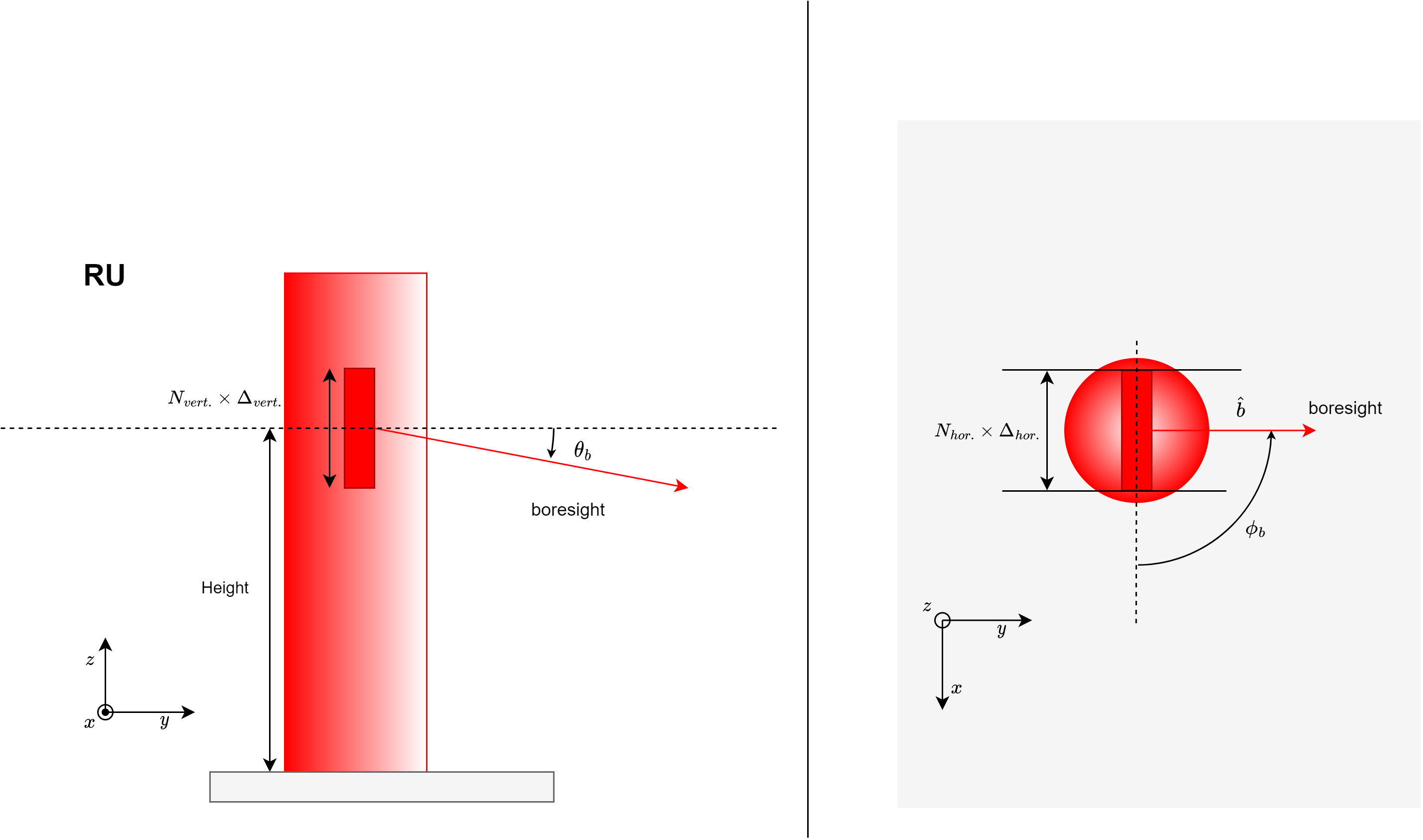
- Horizontal Elements (\(N_{hor.}\)): the number of elements in a row of the planar antenna array.
- Horizontal Spacing [mm] (\(\Delta_{hor.}\)): this field represents the uniform horizontal spacing used in the planar antenna array.
- Vertical Elements (\(N_{vert.}\)): the number of elements in a column of the planar antenna array.
- Vertical Spacing [mm] (\(\Delta_{vert.}\)): correspondingly, this other field indicates the uniform vertical spacing.
- Roll of First Pol. Element [deg]: this field expresses the roll angle, with respect to the vertical axis, of the first element in a dual polarized antenna site (e.g., \(0^\circ\)).
- Roll of Second Pol. Element [deg]: the corresponding roll angle for the second element in a dual polarized antenna site (e.g., \(90^\circ\)). Has an effect only when the array is composed of dual polarized elements.

RUs#

This entry in the stage widget collects the deployed RUs, which are added to the scene by right clicking on the viewport area with mouse and selecting Aerial > Deploy RU. By selecting a given RU in the list, we can set two different sets of properties:
- Cell ID: the unique identifier that defines the cell supported by the given RU.
- Distributed Unit (DU) ID: the unique identifier of the DU associated with this RU (see next attribute).
- DU Manual Assignment: if enabled, users can manually override the DU ID for the selected RU. If disabled, the nearest valid DU will be assigned to the RU. If no existing DUs have matching carrier frequency and total number of antennas as the panel the RU makes use of, a new DU with the necessary properties will be created and assigned to the RU.
- Enable Rays: this flag indicates whether the rays shot from a given RU needs to be included in the telemetry visualized after the simulation. For the rays to a given UE to appear, the corresponding field on the UE side also needs to be enabled.
- Height (m): the height of the antenna panel from RU base.
- Mechanical Azimuth (\(\phi_b\)): azimuth of the RU boresight (indicated as \(\hat{b}\) in the figure below).
- Mechanical Tilt (\(\theta_b\)): elevation of the RU boresight (indicated as \(\hat{b}\) in the figure below) with respect to the horizon.
- Panel Type: the specific antenna array for the RU currently selected.
- Radiated power (dBm): the total radiated power, across the whole antenna array, for the given RU.

DUs#

This entry in the stage widget collects the deployed DUs, which are added to the scene by right clicking on the viewport area and selecting Aerial > Deploy DU. When deployed, the DUs are placed above the buildings in its immediate proximity, so it might be necessary to zoom out in order to see them after the deployment. The location of a DU serves as a visual aid to clarify DU-RU associations, rather than representing the actual physical position of a DU on the map. By selecting a given DU in the property widget, we can set:
- Aerial Properties
- ID: the unique identifier for this DU.
- Carrier Frequency [MHz]: the center frequency that the assigned RU panels are expected to emit at.
- Max Channel Bandwidth [MHz]: the largest bandwidth supported by the DU. This RAN-specific field is currently read-only. Editing functionality will be added in future updates.
- Number of Antenna Elements: the number of antennas that the panels assigned to associated RUs are expected to make use of.
- Sub-carrier Spacing: parameter indicating the spectral distance between two adjacent sub-carriers in the OFDM waveform used by the RU.
- Waveform FFT size: the size of the FFT used in the orthogonal frequency division multiplexing (OFDM) waveform. This parameter is used when Enable Wideband CFRs or Simulate RAN are active in Scenario.
Please note the following when assigning an RU to a DU:
- Multiple RUs can be assigned to a DU by editing the ID attribute in the RUs.
- All RUs belonging to a DU must have the same number of antennas where num_ants = num_horizontal_elements * num_vertical_elements * num_polarizations.
- When a RU is created, the UI will attempt to associate it with the closest DU if the RU satisfies the above requirements.
- Users can manually associate RUs to DUs which are further away than the one in direct proximity as long as the RUs satisfies the above requirements.

Scenario#

This entry in the stage widget collects all the simulation parameters that can be currently set. This includes:
- Default UE panel: this is the antenna array associated by default to any UE in the simulation. As we will see later, this parameter can be overridden locally.
- Default RU panel: same concept as described for the default UE panel, but for the RU panel.
- Simulate RAN: enables the possibility of simulating the behavior of the deployed RUs by adding a physical layer and a medium access control layer to both RUs and UEs.
- Simulation mode: when Simulate RAN is disabled, this field allows to choose between two different ways of specifying the simulation timeline. In Slots mode, the simulation timeline is described by the number of slots per batch and the number of realizations of the channel per slot (Samples per Slot). Differently, in Duration mode, the timeline is described by a total temporal length of simulation (Duration) and the sampling period across said duration is set by Interval. If Simulate RAN is enabled, only Slot mode is possible.
- Duration (s): this number represents the amount of simulated time for which we would like to generate realizations of the radio environment.
- Interval (s): this parameter indicates the sampling period with which the radio environment is to be sampled. Limited to 0.1s when Urban Mobility is enabled to preserve simulation trajectory.
- Number of Batches: the number of UE redrop events during the simulation. This parameter is useful when training neural networks. The evolution of the UEs movement is smooth and gradual. Correspondingly, the statistics of the channel does not change appreciable if not across many samples. Thanks to this parameter, it is possible to accelerate the convergence of the training process by UEs redropping, which occur for every batch.
- Slots per Batch: number of slots to simulate for every batch in the simulation. The total number of batches in the simulation is specified in Batches.
- Samples per slot: number of samples to consider in a given slot. This field can either be 1 or 14, indicating whether or not the simulation should account for the Doppler effect within a slot.
- EM Diffusion: indicates how a surface scatters light, either uniformly in all directions (Lambertian) or with a directional bias.
- Enabled Wideband CFRs: this flag indicates whether channel frequency responses are also going to be generated.
- Emitted rays: this is the number of emitted rays at a given RU in thousands.
- Max Paths: this is the average number of paths used in simulations and saved in for every link in the ClickHouse database.
- Ray Bounces: the total number of admissible scattering events along any of the traced rays.
- Enable Temperature Color: this flag indicates whether the rays need to be colored based on their power.
- Max dynamic range (dB): the power range in dB that should be considered for the visualization of the rays. This range sets the power threshold - from the strongest ray - under which the graphical interface will omit the visualization of rays.
- Max Visible Ray Paths Per RU-UE: this field sets the number of visualized rays per RU-UE pair.
- Ray sparsity: whilst the RAN digital twin calculates the rays for all temporal samples, this field allows to only propagate a fraction of such rays to the graphical interface. This is convenient when running long simulations, which would require the transfer of substantial amount of data towards the graphical interface, which will have to keep the data in RAM. E.g., a Ray sparsity factor of 10 means that the graphical interface will only request the rays once every 10 samples.
- Ray Width (cm): the diameter of the ray curve on the map.
- Enable Seeded Mobility: indicates whether the random number generators involved in the creation of UE mobility are seeded or not.
- Mobility Seed: in case the previous parameter is set to true, this indicates the seed for the random number generators.
- Enable Urban Mobility: enables geospatially informed mobility instead of a procedural mobility model. Required for dynamic scatterers. Speed of dynamic scatterers and UEs will also be geospatially informed, based on road network speed limits. This feature is experimental for now and the results could different from the expectation of the users in release 1.3.
- Number of procedural UEs: this indicates how many procedural UEs will be present during the simulation. Currently limited to a maximum of 2000. If Enable Urban Mobility is checked, this parameter is considered as maximum number of procedural UEs. There is currently no guarantee that the parameter will be enforced.
- Indoor Procedural UEs: the percentage of indoor procedural UEs relative to all procedural UEs that will be present during the simulation.
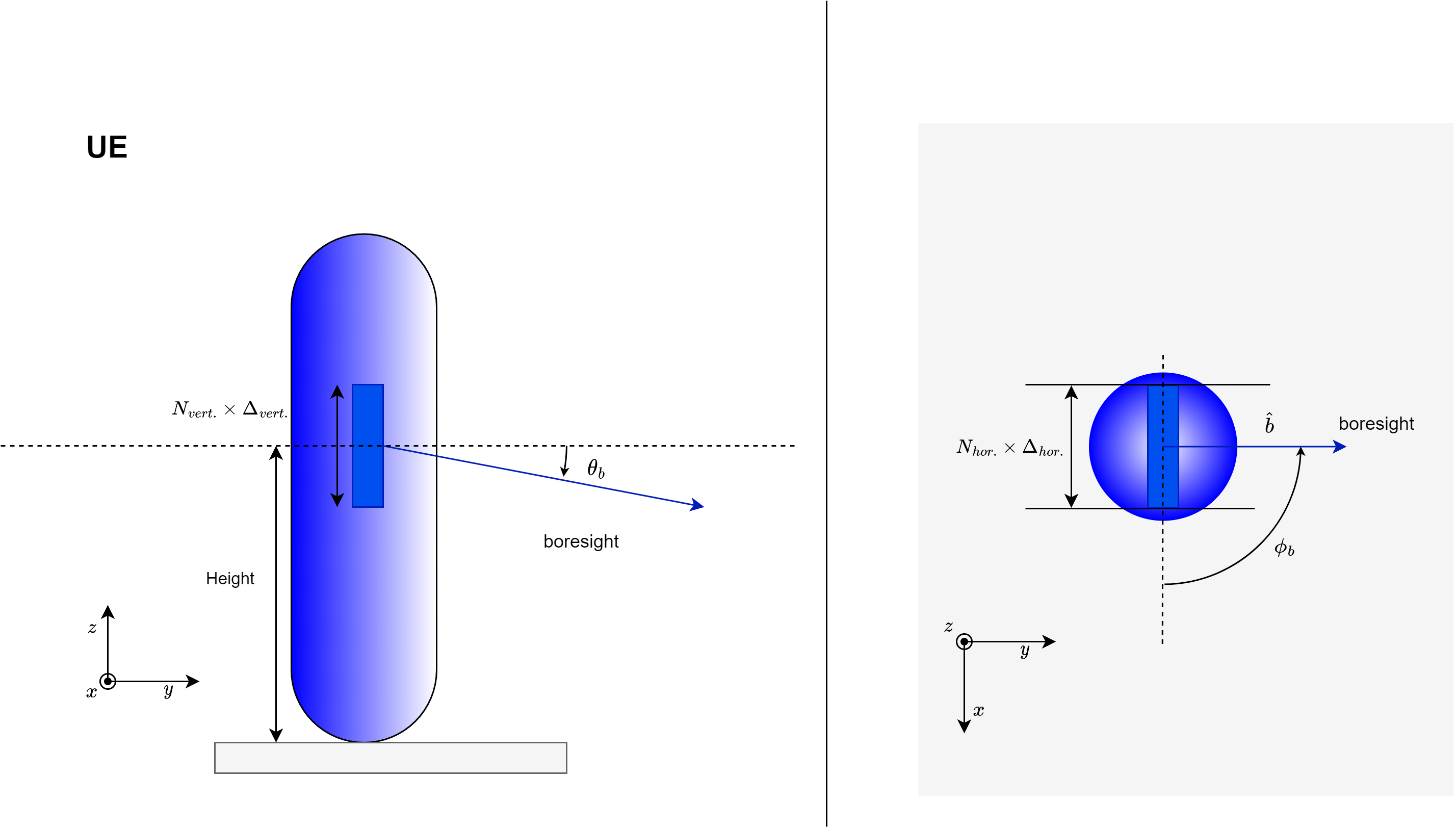
- Capsule Height (m): the UE height which will be applied to all UEs in the scene.
- Capsule Radius (m): the radius of the spheres at the UEs’ position for the purpose of finding the propagation paths in the ray tracing of the EM engine.
- Max Speed (m/s): the maximum speed of the UEs in the simulation.
- Min Speed (m/s): the minimum speed of the UEs during the simulation. The actual speed of given UE will be picked from a uniform distribution going from UE Min speed to UE Max speed.
- Enable Dynamic Scattering: enables dynamic scatterer generation on the stage. If toggled while scatterers are on the stage, they will be removed. Requires Urban Mobility to be enabled.
- Max Number of Vehicles: the maximum number of vehicles to simulate. Actual number of vehicles may be lower than requested due to road capacity or simulation conditions. As of release 1.3, this parameter can at most be 50. Moreover, to get closer to such a number, without artifacts, it is important that spawn zone is as large as possible. This limitatation will be removed in future releases.
- GPX File Paths: allows for the import of a GPX trace. Multiple GPX traces may be selected.

UEs#

Once a UE is deployed, using either the viewport context menu (Aerial > Deploy UE) or the programmatic approach described next, the UE will be found under the scope of this entry. By selecting a given UE, we can configure two different sets of properties:
- ID: the unique identifier that distinguishes a given UE from the others.
- BLER Target: the desired block error rate for the UE. This value represents the target rate of errors in transmitted transport blocks and is used to guide adaptive modulation and coding schemes.
- Enable Rays from: this field indicate the list of the RUs whose rays will be included in the UE-specific telemetry visualized after the simulation. For the rays from a given RU to appear the corresponding field needs to be enabled on the RU side.
- Manually Created: this flag indicates whether UE has been positioned directly by the user, or it has been generated procedurally by the software.
- Mechanical Tilt (\(\theta_b\)): elevation of the UE boresight (indicated as \(\hat{b}\) in the figure below) with respect to the horizon.
- Panel Type: the specific antenna array for the UE currently selected.
- Radiated power (dBm): the total radiated power, across the whole antenna array, for the given UE.

runtime#

The runtime prim collects the trajectories along which the UEs will move during the simulation after UE have been generated.

World#

This entry contains the geometry describing the scene.

Scatterers#

Scatterers are the non-UE dynamic elements in the simulation. Once mobility is generated, the following hierarchy is established:
- Vehicles
  - By selecting the mesh used to represent the vehicles, the following properties can be configured for all vehicles on the stage:
    - Diffuse Surface Element Area: average area of the diffuse surface element.
    - Enable RF: this flag indicates whether vehicle meshes on the stage can interact with the electromagnetic field. If this flag is not enabled the electromagnetic field will not be able to interact with the geometry of the selected asset. Enabled by default.
    - Enable Diffusion: this option in turn specifies whether vehicle meshes on the stage can interact with the electromagnetic field in a diffuse fashion, i.e., whether the surface of such meshes can produce non-specular reflections.
    - Surface Materials: this selects the surface material associated with all scatterers present on the stage.

9. Timeline widget#

The timeline widget allows the user to manually move across the simulation once the EM solver has calculated the radio frequency (RF) environment. This can be accomplished moving the marker across the timeline.

The numbers along the timeline represent frames. The total frame count is calculated as \( \dfrac{24 × \rm{simulation \ duration}}{\rm{sampling \ interval} } \) when the RAN is not simulated, where the sampling interval is defined in the Scenario entry of the stage widget. When the RAN is simulated, the frame count instead equals the number of \( 24 \cdot \left(\rm{slots}-1\right) \cdot \rm{symbols \ per \ slot} + 24 \cdot \left(\rm{symbols \ per \ slot} - 1\right). \) If batches are present, the timeline is expanded across them. The total number of frames is refreshed each time the Generate Mobility button (described above) is clicked. In release 1.3, a multiplier of 24 is applied by default due to an application constraint on the number of time codes per second. As a result, a single time sample from UEs, vehicles, or rays spans 24 time codes, with the translate attribute of UEs and vehicles interpolated between consecutive samples across such codes.