RAN Digital Twin#
The following sections describe how to run simulations in two different modes:
Mode 1 - Electromagnetic Only (EM): compute radio propagation using ray tracing
Mode 2 - Radio Access Network (RAN): run AERIAL 5G RAN protocols in addition to the EM simulation
Simulation Mode 1 - EM Simulation#
The EM simulation mode simulates the electromagnetic propagation between transmitters and receivers in a virtual 3D environment. It generates the wireless channel between them, but does not execute any component of the RAN. As such, it can be used to create large quantities of synthetic data, which can be accessed through SQL for further processing.
Both modes of operation require some common steps:
Attaching worker - a worker is a node that performs computations (such as ray tracing, channel emulation, antenna modeling, as well as running the RAN). The worker communicates with the UI via the Nucleus and NATs servers.
Creating and configuring antenna panels
Deploying network components (RUs and DUs)
Deploying UEs and configuring their mobility patterns or spawn settings
Configuring raytracing simulations and executing them.
These steps are described in more detail below.
Attaching a worker to the UI#
As discussed in the previous sections, the Aerial Omniverse Digital Twin consists of six subcomponents:
the graphical user interface
Nucleus
ClickHouse
NATS
the scene importer
and the RAN digital twin,
where the Nucleus and the NATS servers are the elements that allow all the others to interact with one another.
Our entry point to running simulations is the graphical user interface. After opening the graphical interface, we can navigate to the Configuration tab to attach to an instance of the RAN digital twin, here referred to also as a worker.
Once in the Configuration tab, we will enter the DB host and DB port for the ClickHouse server. We can also add a DB name and, optionally, a DB author. DB notes can be left empty or used to describe key characteristics of the simulation, which can help us retrieve them later. If the ClickHouse server is successfully reached after pressing the Connect button, the indicator next to it will change from red to green. We can disconnect from the server at any time by clicking the Disconnect button.
Next, we can enter the NATS server path, e.g., localhost, and the desired NATS message subject, which serves as a unique prefix that enables communication with the worker and ensures that multiple workers on the same node remain isolated. By default, the NATS message subject is set to aerial for the EM worker and gis_aerial for the GIS worker. Finally, we will specify the live Session name and the URLs of the Assets installed on the selected Nucleus server.
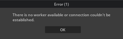
After completing these steps, we are ready to click the Attach Worker button from the toolbar, which is represented by an icon of a set of gears. If there is a problem with the installation and the graphical user interface is unable to communicate with the worker, an error window will appear.
Differently, if the worker attaches successfully, the gear icon will turn green as shown below. To detach the worker, click the gear icon again and confirm that you want to proceed with detaching the worker. The icon will turn gray again.


It is worth mentioning that it is not necessary to explicitly connect to the database each time, as attaching the worker will also establish a connection to the database. Of course, the DB host and DB port must be valid for this to occur.
After attaching the worker, we are ready to open a scene. We can do so by going to File > Open and selecting a scene, e.g., tokyo.usd. Alternatively, we can use the Content tab and double-click on the file we want to open.
After the UI and the worker both open the scene, a 3D map will appear in the viewport, and the Live session icon in the top right will turn green, indicating that the live session is active.
Adding antenna panels#
Next, we need to create the antenna panels that the RUs and UEs will use. We can create a new antenna array by right-clicking on the Stage widget and selecting the Aerial > Create Panel entry from the context menu. The new panel can be found in the Stage widget, under the Panels entry. By choosing the new panel, we can inspect its properties and change them using the Antenna Elements tab and the Property widget, as illustrated in the figure below.
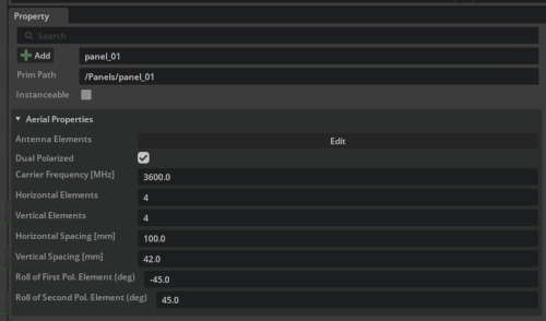
If needed, under the Antenna Elements tab, for half-wave dipoles, it is possible to calculate the active element pattern for each antenna element in the array using the Calculate AEP feature. This takes into account the mutual coupling effects that each antenna element experiences due to the presence of the others. Refer to the Graphical User Interface section of this guide for more information on deploying custom antenna patterns.
Deploying RUs#
To deploy new radio units (RUs), right-click on the map with the mouse and select Aerial > Deploy RU. This will create a movable asset that follows the mouse. Once the location of the RU is found, we can click to confirm the RU’s position. The RU can be later moved by selecting it and moving it with the Move button in the toolbar. After a given RU is in the intended position, its attributes can be modified using the property widget. Most importantly, we need to associate a Panel Type if the field is empty.
Deploying DUs#
To deploy a distributed unit (DU), we can right-click on a map area and select Aerial > Deploy DU. We can manually or automatically associate a DU with an RU. For more details, refer to the Graphical User Interface section of this guide.
Deploying UEs#
The UEs can be deployed in the following ways:
Manually#
To deploy manually, navigate to the viewport and right-click on the position where you would like the UE to be located. Selecting Aerial > Deploy UE from the context menu will create a capsule in the desired location. The corresponding entry in the UEs group of the stage widget will have the Manually Created flag active.
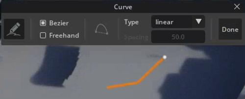
For a manually created UE, we can also specify its mobility by clicking the Edit Waypoints button in the UE property widget and drawing a polyline in the viewport to represent the intended trajectory of the UE across the map.

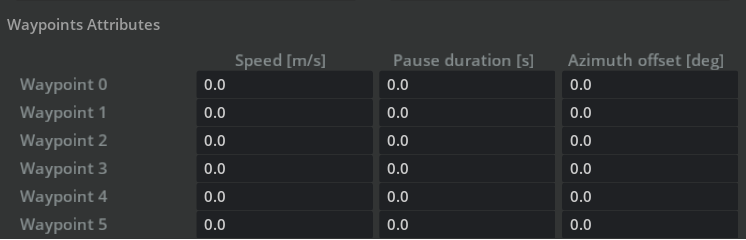
Additionally, the following properties can be customized for each manually drawn waypoint:
Speed: defined in meters per second.
Azimuth angle offset: measured in degrees.
Pause duration: length of time, in seconds, the UE loiters at the waypoint.
This approach is typically sufficient to simulate small scenarios, where the number of UEs is limited.
Procedurally#
For larger populations of UEs, we can procedurally generate them by changing the Number of Procedural UEs parameter in Scenario. Another parameter, Percentage of Indoor Procedural UEs, controls the percentage of procedurally generated UEs that are placed indoors. Note that manual UEs cannot be deployed indoors. Pressing the Generate Mobility button in the toolbar, when the worker is attached, will procedurally create enough UEs so that the number of procedurally generated terminals matches the one specified in Scenario. If Number of Procedural UEs is lower than the existing number of procedural UEs, the additional procedural UEs will be deleted to match the setting.
We can also constrain where the procedural UEs are generated by creating a spawn zone. To do this, right-click in the viewport and select Aerial > Deploy Spawn Zone.
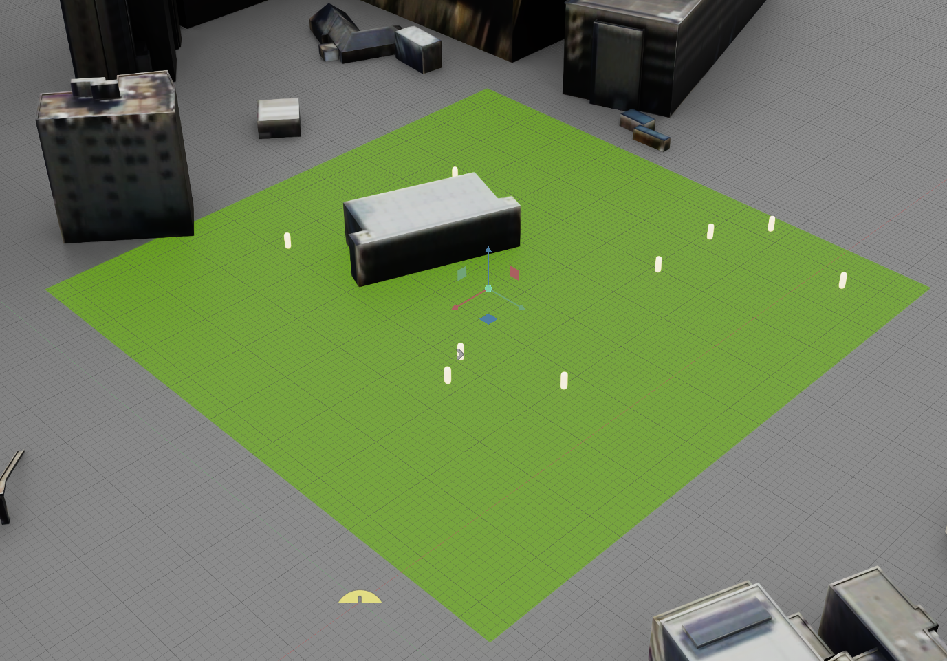
The size and position of the plane can be adjusted using the Move, Rotate, and Scale buttons in the toolbar.
If there is no spawn zone or if the spawn zone is too small, then procedural UEs will be dropped in a random position in the scene. Procedural and manual UEs can be mixed for a given deployment, and manual UEs are not moved at every press of the Generate Mobility button.
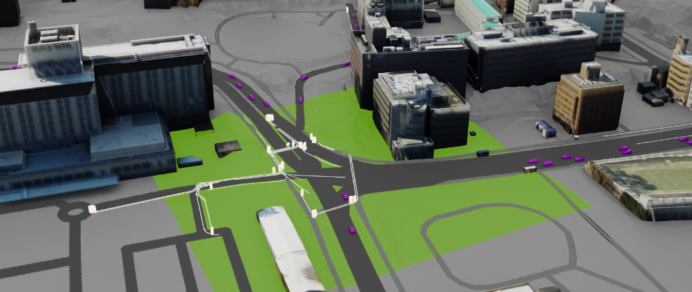
Urban Mobility#
From release 1.3.0, it is also possible to use an experimental behavioral model for procedurally generated UEs by checking the Enable Urban Mobility box. This constrains the trajectories of the UEs to sidewalks, crosswalks, and other pedestrian infrastructure. When used with the Enable Dynamic Scatterers flag, which enables electromagnetic scattering from the vehicles, the model allows for the simulation of consistent UE and vehicular mobility, with full support for the electromagnetic characterization of the field due to the moving cars.
Urban Mobility requires a spawn zone to define the road network data obtained from OpenStreetMaps (OSM). The imported road network creates the area used by the simulation. Any road or sidewalk element that intersects or touches the spawn zone will be included. It is therefore possible for a road element to extend beyond the spawn zone, and as a result, the UE and vehicle trajectories may do so as well.
The simulation logic for Urban Mobility is based on SUMO (Simulation for Urban Mobility)[1]. SUMO derives the road network for simulations from the road network imported from OSM. Using this domain and knowing the requested number of UEs and vehicles, SUMO:
Simulates the trajectories of UEs and vehicles, ensuring that cars avoid collisions with UEs and other vehicles.
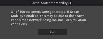
Automatically adjusts the number of vehicles if the road network’s vehicular infrastructure reaches capacity. Cars that cannot complete a trajectory of the desired duration or fit within the simulation are removed, with a notification in the UI.
Generates no UE if the spawn zone’s Urban Mobility domain lacks pedestrian infrastructure.
As of release 1.4.0, the integration with SUMO includes a few caveats, e.g.
In the case that the value of Max number of Vehicles in Scenario cannot be supported by the spawn zone’s road network, a fewer number of vehicles may be generated.
To ensure a constant number of vehicles in the scene, vehicles may be rerouted if their trajectory reaches a dead end or ends before the value of Duration in Scenario.
If the SUMO generated fewer vehicles or UEs than requested, a notification appears in the UI.
Even so, however, consistency and repeatability are ensured, and Enable Seeded Mobility and Mobility Seed are respected.
GPX Import#
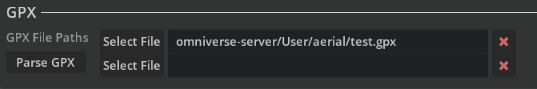
Additionally, UEs can be created out of GPX traces. After selecting the desired GPX files in Scenario, click the Parse GPX button to create a manual UE for each trace. Once the UEs are created, clicking Generate Mobility will generate trajectories that match the data contained in the GPX files.
When using GPX traces, the simulation duration determines how the trajectory is handled:
If the simulation duration exceeds the length of the GPX trace, the procedural mobility model will take over once the GPX trace waypoints are exhausted.
If the simulation duration is shorter than the length of the GPX trace, the trajectory of the manual UE will be truncated to match the specified duration.
Changing the scattering properties of the environment#
The proper association of materials to the scene geometry plays a key role in producing a realistic representation of the radio environment. Currently, materials can be assigned to each building and to the terrain as a whole. To do so,
we can select the exterior part of a building we want to edit using either the stage view or the viewport, and then proceed to alter the Surface Materials fields in the property widget; we can similarly select the building in the stage view and edit the Surface Materials field for the interior part of the building.
For the terrain, we can select the Ground Plane asset in the Stage view and then modify the Surface Materials field in the Property widget.
For the buildings, it is also possible to batch assign a given material to the entire map by selecting /World/buildings in the stage widget.
With a similar procedure and interface, we can also assign :
Enable RF: this flag indicates whether the mesh or meshes representing
one building,
all of the buildings
or the terrain
can interact with the electromagnetic field. If this flag is not enabled, the electromagnetic field will not be able to interact with the geometry of the selected asset;
Enable Diffraction: this flag indicates whether the meshes can interact with the electromagnetic field through diffraction.
Enable Diffusion: this option specifies whether the mesh or meshes can interact with the electromagnetic field diffusely, i.e., whether the surface of such meshes can produce non-specular reflections.
Diffuse Surface Element Area: finally, this parameter specifies the area of the tiles in which the surfaces of given meshes will be represented in the calculation of the diffusive electromagnetic components. This parameter allows control of the number of rays diffused by a single facade.
Running simulations#
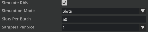
Before running the simulation, it is essential to verify that all parameters in the Scenario property widget align with our intentions and that the Simulate RAN checkbox is unchecked.
As mentioned in the previous section, the duration and the sampling period of the simulation are determined by the Simulation Mode in Scenario.
Simulation Mode: Duration requires setting
Batches,
Duration,
Interval
Simulation Mode: Slots instead requires
Batches,
Slots Per Batch,
Samples Per Slot.
Refer to the Graphical User Interface section, which describes the Scenario stage widget, for more details on these and other parameters.
Once we have the parameters correctly set, we can generate the UEs and their corresponding trajectories using the Generate UEs button. The trajectories appear in the viewport widget as white polylines on the ground plane, and in the Stage widget as entries of the runtime scope. Once the UEs and their trajectories are available, we can start the simulation by pressing the Start UE mobility button in the toolbar.
While running, the simulation can be paused and stopped using the Pause Mobility and the Stop Mobility buttons of the toolbar. While the simulation is paused, the Generate Mobility button can be pressed but it will not generate a new set of trajectories. In order to so, the simulation will have to be stopped using the Stop Mobility button. The progress of the simulation is shown in the progress bar.

Headless operation#
After Generate mobility is pressed, a database containing the necessary information to run the simulation is saved and stored on the ClickHouse server. At this point, the graphical interface can be closed and the simulation can be launched directly from the aodt_sim container.
cd <path to aodt backend installation> # e.g. ~/aodt_1.3.1/backend
aerial:~/aodt_1.3.1/backend$ docker compose exec -it connector bash

# note command line options
aerial:/aodt/aodt_sim/build$ python -m aodt.app.sim --help

# replay simulation from a database (note your nucleus and clickhouse hostnames may be different)
aerial:/aodt/aodt_sim/build$ python -m aodt.app.sim --nats_server_url="omniverse://omniverse-server" --nats_subject="aerial" --db-host clickhouse --db-replay --db-name-source <database name, e.g. aerial_2025_1_7_16_40_42>

# run without entering the container (can be used to run several databases via a script)
docker compose exec connector python -m aodt.app.sim --nats_server_url="omniverse://omniverse-server" --nats_subject="aerial" --db-host clickhouse --db-replay --db-name-source <database name>
Starting from release 1.3.0, it is possible to initiate a simulation without using the graphical interface at all. All parameters, including the location of RUs and UEs, can be specified using a YAML file. From the aodt_sim container, we can
# simulate from scratch with configurations specified in --sim-config
aerial:/aodt/aodt_sim/src_py$ python -m aodt.app.sim --log=<log level> --nats_server_url=<path to NATs server> --nats_subject=<NATs subject> --db-replay --db-host=<path to clickhouse server> --db-name-source=<source database created from the yml file> --sim-config=<path to config file in .yml>
or, alternatively
# simulate a source database and save to a new destination database with updated parameters specified in --sim-config
aerial:/aodt/aodt_sim/src_py$ python -m aodt.app.sim --log=<log level> --nats_server_url=<path to NATs server> --nats_subject=<NATs subject> --db-replay --db-host=<path to clickhouse server> --db-name-source=<source database from which to replay> --db-name-destination=<new database to write results into> --sim-config=<path to config file in .yml>
The --db-name-destination argument is optional and defaults to the source database, and --sim-config is used to specify the YAML config file. See the headless simulation configuration section for the details.
Server-Client operation#
In addition to headless operation, the digital twin can run in server-client mode, where a service performs EM computations and a C++ or Python (through bindings) client consumes the computed channels realizations. This architecture enables clients to access GPU memory directly for efficient data sharing.
The server-client mode is particularly useful for providing with external simulators or applications with highly accurate realizations of the wireless channel.
To start the digital twin service, install AODT and run the following from the developer container (see Source code and dev. container for setup details):
# Start the digital twin service
aerial:/aodt/aodt_sim/src_py$ OMNI_USER=omniverse OMNI_PASS=aerial_123456 \
    python -m aodt.app.sim \
    --nats_server_url=<path to NATs server> \
    --nats_subject=<NATs subject> \
    --db-host=<path to clickhouse server> \
    --db-name-source=<source database> \
    --log=debug \
    --dt-server \
    [--dt-server-port 50051]
The --dt-server flag enables the gRPC server. The --dt-server-port parameter is optional (default: 50051). Once the server is running, clients can connect to it and provide their YAML configuration (which can be generated programmatically or loaded from a file) to initialize scenarios and request channel computations for specific time steps, RUs, and UEs.
The typical workflow involves:
Define Scenario: Define the scenario configuration as a YAML string, either by generating it programmatically (See headless simulation configuration) or loading from a YAML file.
Start: The client loads the YAML configuration and starts the scenario on the server. At this stage, we can query the positions of the RUs or of the UEs and allocate the GPU memory to store the CIR results. Subsequently, we can enter a time loop.
Loop: For each time step:
Compute CIR using the EM solver
Access CIR data via zero-copy from GPU or by copying from GPU to host
Process the channel data At the end of the loop, we can finally deallocate the reserved GPU memory.
See the Server-Client API reference section for detailed API documentation and usage examples.
Viewing simulation results#
At the end of a simulation, or after loading an existing database by doube-clicking on its name in the Configuration tab, we can press the Play button on the toolbar or move the blue indicator in the Timeline widget to a specific frame of interest. To stop the replay, we can click the Stop button.
The visualization of the rays can be turned on or off for each RU-UE pair by selecting the UE and enabling the Show Raypaths attribute in the Property widget. If a given RU was not chosen before the simulation was launched, and we are interested in seeing the rays of that RU-UE pair, we can use the Refresh telemetry button.
Radio environment#
The radio environment results stored in the database are for the downlink direction, i.e., from the RU to the UE. Specifically, if we take
the total transmitted power \(P^{\left(RU\right)}\) at RU,
the number of polarizations used at RU per transmitting antenna site \(N^{\left(RU\right)}_{pol.}\)
the number of horizontal antenna elements used at the RU \(N^{\left(RU\right)}_{hor.}\)
the number of vertical antenna elements used at the RU \(N^{\left(RU\right)}_{vert.}\)
the number of FFT points \(n\)
the channel frequency response per link \(\mathbf{H}_{i,j}^{\left(UE\right)}\left( k \right)\) observed at the UE for a given subcarrier \(k\), across the link from the \(i\)-transmitter antenna to the \(j\)-th receiver antenna
the channel frequency response per link \(\mathbf{H}_{i,j}^{\left(ch\right)}\left( k \right)\) observed at the UE for a given subcarrier \(k\), across the link from the \(i\)-transmitter antenna to the \(j\)-th receiver antenna when each subcarrier is allocated unitary power at transmission
the results are such that
\( \left<\mathbf{H}_{i,j}^{\left(UE\right)}, \mathbf{H}_{i,j}^{\left(UE\right)} \right> = \dfrac{P^{\left(RU\right)}}{n \cdot N^{\left(RU\right)}_{pol.} \cdot N^{\left(RU\right)}_{hor.} \cdot N^{\left(RU\right)}_{vert.}} \left<\mathbf{H}_{i,j}^{\left(ch\right)}, \mathbf{H}_{i,j}^{\left(ch\right)} \right>. \) The set of \(\left\{\mathbf{H}_{i,j}^{\left(UE\right)}\left( k \right)\right\}_{i,j,k}\) is stored in the cfrs table discussed in the next section.
If we define \( \mathbf{h}_{i,j}^{\left(UE\right)} = \dfrac{{\rm{iFFT}}_n \left[ \mathbf{H}_{i,j} ^ {\left( UE \right)}\right]}{\sqrt{n}} \) and the geometrically calculated channel impulse response as \( h^{UE}_{i,j} \left(t\right) = \sum_w h^{\left(w \right)}_{i,j} \delta\left(t - \tau^{\left(w \right)}_{i,j} \right) \) we also have \( \left<h^{UE}_{i,j}, h^{UE}_{i,j}\right> = \left<\mathbf{h}_{i,j}^{\left(wb\right)}, \mathbf{h}_{i,j}^{\left(wb\right)}\right> \) where the set of \(\left\{h_{i,j}^{\left(UE\right)}\right\}_{i,j}\) is stored in the raypaths table discussed in the upcoming section.
Finally, if we are interested in calculating the channel frequency response in uplink, we can do so by imposing \( \left<\mathbf{H}_{i,j}^{\left(RU\right)}, \mathbf{H}_{i,j}^{\left(RU\right)} \right>_{UL} = \dfrac{P^{\left(UE\right)}}{N^{\left(UE\right)}_{pol.} \cdot N^{\left(UE\right)}_{hor.} \cdot N^{\left(UE\right)}_{vert.}} \cdot \dfrac{N^{\left(RU\right)}_{pol.} \cdot N^{\left(RU\right)}_{hor.} \cdot N^{\left(RU\right)}_{vert.}}{P^{\left(RU\right)}} \left<\mathbf{H}_{i,j}^{\left(UE\right)}, \mathbf{H}_{i,j}^{\left(UE\right)} \right>_{DL}. \)
Simulation Mode 2 - RAN simulation#
The RAN simulation mode builds upon the EM mode and adds key elements of the physical (PHY) and medium access control (MAC) layers. As for the previous mode, all data capturing the detailed interaction between RAN and UEs can be accessed through SQL for further processing or analysis.
To enable the simulation of the RAN, select the Scenario entry under the Stage widget and enable the Simulate RAN checkbox, as shown in the figure below. This will restrict the Simulation mode field to Slots.
We can then define the number of batches, number of slots per batch and samples per slot as in EM mode. Specifically,
when
Samples Per Slotis set to 1, a single front-loaded realization of the channel will be used across the whole slotwhereas, when
Samples Per Slotis set to 14, every OFDM symbol will be convolved with a different channel realization.
If the RUs are configured with a 64-antenna panel in the RAN simulation, MU-MIMO is enabled in MAC scheduling. The reader can refer to the MAC Scheduling section for a detailed description and the RAN Parameters table for relevant parameters.
RAN Parameters#
The RAN parameters are stored in
/aodt/aodt_sim/src_be/components/common/config_ran.json
where the following parameters can be changed
Meaning |
Default value |
|
|---|---|---|
gNB noise figure |
Noise figure of RU power amplifier. |
0.5 dB |
UE noise figure |
Noise figure of UE power amplifier. |
0.5 dB |
DL HARQ enabled |
Enables DL HARQ. |
0 |
UL HARQ enabled |
Enables UL HARQ. |
0 |
TDD patterns |
Supported TDD patterns, additional patterns can be added. |
1: DDDSUUDDDD |
Simulation pattern |
Specifies the TDD pattern for simulation. |
1 (i.e., DDDSUUDDDD) |
Max scheduled UEs per TTI - dl |
Maximum number of UEs per TTI per cell for DL. |
6 (max: 6) |
Max scheduled UEs per TTI - ul |
Maximum number of UEs per TTI per cell for UL. |
6 (max: 6) |
Scheduler Mode |
Specifies the PRB scheduling algorithm. Options: “PF” (proportional fairness scheduler) or “RR” (round robin scheduler). |
“PF” |
Beamformers CSI |
Specifies the CSI for beamforming. Options: “SRS” (SRS estimated channels) or “CFR” (ground truth channels). |
“CFR” |
MAC CSI |
Specifies the CSI for L2 MAC scheduling. Options: “SRS” (SRS estimated channels) or “CFR” (ground truth channels). |
“CFR” |
Beamforming Grp Level |
Specifies beamforming group level. Options: “SC” (per subcarrier beamforming), “PRBG” (per PRBG beamforming), or “UEG” (per UEG beamforming). |
“PRBG” |
pusch channel estimation |
Specifies the method for estimating the. Options: “MMSE”. |
“MMSE” |
srs channel estimation |
Specifies the method for estimating the. Options: “MMSE” or “RKHS”. (“RKHS” is only supported with 64 antennas at the RU). |
“MMSE” |
channel estimation duration |
Specifies the delay spread window size for MMSE channel estimation. Options: 1 (1 us) or 2 (2 us). |
2 |
MCS selection mode |
Specifies the method for MCS selection. Currently, only “OLLA” (Outer Loop Link Adaptation) is supported. |
“OLLA” |
SRS SNR threshold for MU-MIMO feasibility - dl |
Applies when 64 antennas are at the RU. Specifies the SRS SNR threshold to determine if a UE qualifies for MU-MIMO grouping in DL. |
-3 dB |
SRS SNR threshold for MU-MIMO feasibility - ul |
Applies when 64 antennas are at the RU. Specifies the SRS SNR threshold to determine if a UE qualifies for MU-MIMO grouping in UL. |
-3 dB |
Channel correlation threshold for MU-MIMO grouping - dl |
Applies when 64 antennas are at the RU. Specifies the channel correlation threshold for making MU-MIMO grouping decisions in DL. |
0.7 |
Channel correlation threshold for MU-MIMO grouping - ul |
Applies when 64 antennas are at the RU. Specifies the channel correlation threshold for making MU-MIMO grouping decisions in UL. |
0.7 |
Fixed UE layers - dl |
If “Enable Fixed Layers” is set to 1, UEs are always assigned the number of layers specified by the “Fixed Layers” parameter in DL. |
“Enable fixed layers”: 0 |
Fixed UE layers - ul |
If “Enable Fixed Layers” is set to 1, UEs are always assigned the number of layers specified by the “Fixed Layers” parameter in UL. |
“Enable fixed layers”: 0 |
RX FT filename |
If a filename is provided, the received I/Q samples at the receivers will be saved to an H5 file with the specified filename. |
default: “” (disabled) |
Currently, only a portion of the RAN parameters is available for modification in a convenient JSON file. Subsequent releases, however, will include the whole gamut of configuration parameters for all blocks in the RAN.
Simulation#
After the parameters described in config_ran.json are set, we can run the simulation using the same sequence as the EM mode. The results are then propagated to
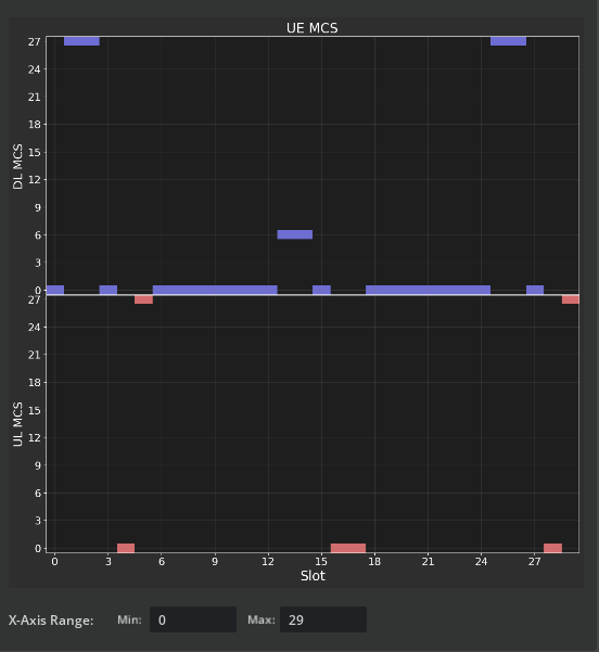
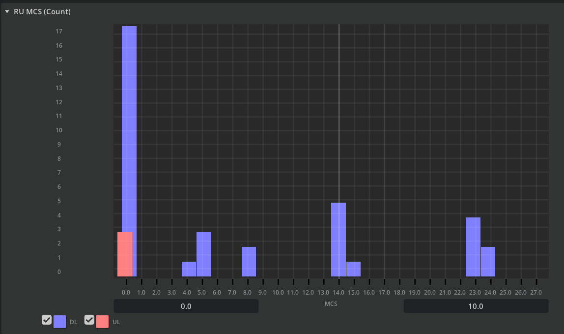
the graphical interface, where we can visualize instantaneous throughput and modulation coding scheme (MCS) for each UE or the RU-level throughput and statistic distribution of the allocated MCSs;
the local console, where detailed scheduling information (e.g., PRB allocations and number of layers) are printed slot-by-slot;
the selected ClickHouse database, where the full telemetry will be stored.
Graphical user interface#
After the simulation is complete, we can select a specific UE or RU under in the Stage widget and press the play button from the toolbar. In the Property widget, we will see the time series of
the instantaneous throughput for UEs,
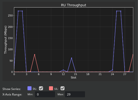
the aggregate instantaneous throughput for the RUs.
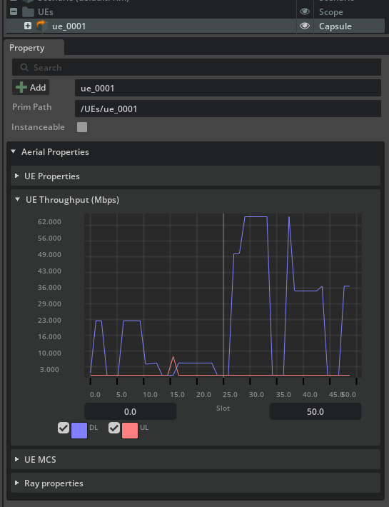
Additionally, we can observe the instantaneous throughput of the UE directly above their representation in the viewport, as shown below.
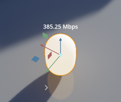
The MCS allocated by the MAC scheduler for a given UE can also be found right below the instantaneous throughput.
Similarly, at the RU, we can find the histogram of the modulation and coding schemes in use across the simulation.
Local console#
If accessible, additional details can be observed in the console where the RAN digital twin is running. At the end of each slot, a table is printed listing all scheduled UEs, PRB allocations (start PRB index and number of allocated PRBs), MCS, number of layers, redundancy version in presence of HARQ, pre-equalization SINR, post-equalization SINR, and CRC results, with 0 denoting a successful decoding.
==============================================  results  ================================================
cell idx   grp idx   ue id     startPrb     nPrb    MCS   layer     RV   sinrPreEq    sinrPostEq     CRC
   0         0         94       176          80       4      2       0     5.67         4.16           0
   0         1         95         4          36       0      2       0    -3.94        -2.43           0
   0         2        155        40          40       3      2       0     1.47         1.10           0
   0         3        175        80          96      27      1       0    34.94        40.00           0
   0         4        192       256          16       1      1       0    -6.14        -1.21           0
   0         5        193         0           4      26      2       0    36.21        26.23        9860658
   1         6         28       200          16      15      1       0    10.12        16.60           0
   1         7         58       216          56      10      1       0     3.95        10.01           0
   1         8         89         0          80      24      1       0    12.64        22.68        7891203
   1         9         92        80          12      27      1       0    35.69        40.00           0
   1        10        178       148          52      12      1       0     6.74        11.62           0
   1        11        184        92          56       7      1       0     2.02         7.28           0
   2        12         34       244          28      27      1       0    34.56        39.19           0
   2        13         47       124          48      15      1       0     6.36        15.37           0
   2        14         60        16          92      16      1       0     5.22        15.24           0
   2        15         68       172          72       9      1       0     3.41         9.45           0
   2        16        194         0          16      11      1       0     3.72        10.74           0
   2        17        199       108          16       3      2       0     9.68         4.18           0
   3        18         23       200           8      27      1       0    31.78        37.85           0
   3        19         56       208          28      20      1       0    14.68        19.20           0
   3        20         57         0          60       3      1       0    -0.52         5.20           0
   3        21         62        60         140      27      1       0    33.20        37.99           0
   3        22        160       260          12      15      1       0    14.91        20.29           0
   3        23        187       236          24      27      1       0    36.80        39.92           0
=========================================================================================================
ClickHouse database#
Comprehensive telemetry data is available in the telemetry table of the database used for the simulation. For instance,
clickhouse-client

aerial :) select * from aerial_2024_4_16_14_28_33.telemetry

SELECT *
FROM aerial_2024_4_16_14_28_33.telemetry

Query id: e463ec6a-4e11-4197-88e0-8762a630181d

┌batch_id─┬─slot_id─┬─link─┬─ru_id─┬─ue_id─┬─startPrb─┬─nPrb─┬─mcs─┬─layers─┬───tbs─┬─rv─┬─outcome─┬───scs─┐─preEqSinr─┬─postEqSinr─┐
│       0 │       0 │ UL   │     0 │    46 │       28 │  132 │   0 │      1 │   372 │  0 │       1 │ 30000 │  8.948093 │  15.192958 │
│       0 │       0 │ UL   │     0 │    49 │        0 │   28 │   0 │      1 │    80 │  0 │       1 │ 30000 │ 30.305893 │   36.59542 │
│       0 │       0 │ UL   │     0 │    53 │      160 │   24 │   0 │      2 │   141 │  0 │       1 │ 30000 │  35.86527 │   38.16932 │
│       0 │       0 │ UL   │     0 │    94 │      184 │   88 │   0 │      2 │   497 │  0 │       0 │ 30000 │ -2.340038 │    0.19586 │
│       0 │       0 │ UL   │     1 │   124 │        0 │  272 │   0 │      1 │   769 │  0 │       1 │ 30000 │ 11.380707 │   9.841505 │
│       0 │       1 │ UL   │     1 │   124 │        0 │  272 │   9 │      1 │  7813 │  0 │       1 │ 30000 │  8.920734 │  15.117773 │
│       0 │       1 │ UL   │     2 │    34 │        0 │  272 │   0 │      1 │   769 │  0 │       1 │ 30000 │  32.23978 │  37.145943 │
│       0 │       1 │ UL   │     3 │    23 │       20 │  252 │   0 │      1 │   705 │  0 │       1 │ 30000 │ 13.059542 │  23.430824 │
...
where the meaning of each column is explained in the Database schemas.
Important: Several scripts are available to extract information from the database. Example scripts and notebooks can be found in aodt_sim/examples to extract and plot CIRs/CFRs, throughputs, BLERs, scheduling metrics and other datapoints stored in the tables above.
MAC Scheduling#
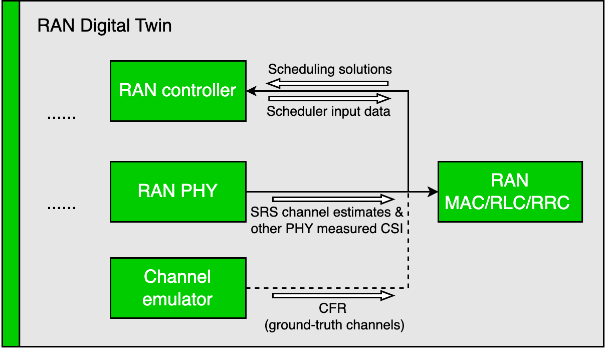
The MAC scheduling tasks are performed by the Aerial cuMAC, with full support for both UL and DL, HARQ, and single-cell as well as multi-cell jointly scheduling. Two different sets of scheduling algorithms are supported for 4T4R SU-MIMO and 64T64R MU-MIMO simulations, respectively:
4T4R SU-MIMO: MAC scheduler pipeline consists of four modules - UE selection, PRB allocation, layer selection, and MCS selection.
64T64R MU-MIMO: MAC scheduler pipeline consists of three modules - MU-MIMO UE sorting, MU-MIMO UE grouping, and MCS selection.
The data flows for the scheduling process are illustrated in the following figures.
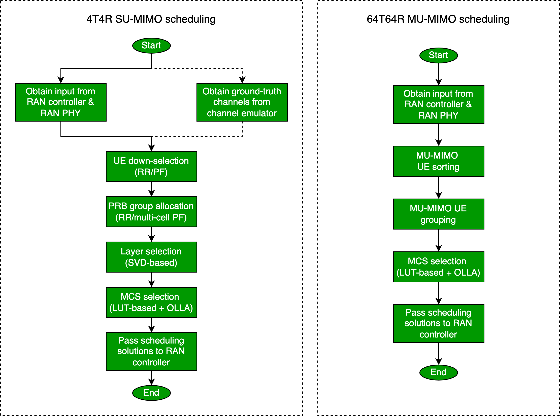
For 4T4R SU-MIMO scheduling, the following procedures are executed in each time slot. First, the necessary input data is provided to cuMAC, and then the four SU-MIMO scheduler functions are run sequentially on the GPU.
UE selection: UE down-selection for each cell using the SINRs measured by the RAN PHY.
PRB allocation: PRB allocation for the selected UEs per cell using either
the SRS channel estimates from the RAN PHY,
or the CFRs (ground-truth channels) from the channel emulator.
Layer selection: layer selection for each selected UE.
MCS selection: MCS selection for each selected UE using the SINR measured by the RAN PHY. Outer-loop link adaptation is used to add a positive/negative offset to the measured SINR. The offset is adjusted based on the ACK/NACK result of the last scheduled transmission for the given UE.
For 64T64R MU-MIMO scheduling, the following procedures are executed in each time slot: first, the necessary input data is provided to cuMAC, and then the three MU-MIMO scheduler functions are run sequentially on the GPU.
MU-MIMO UE sorting: Sorts all active UEs in each cell considering
the proportional-fairness (PF) metrics,
the feasibility of MU-MIMO transmission based on the wideband SRS SNRs measured by the RAN PHY,
and the HARQ re-transmission status.
MU-MIMO UE grouping: for each cell, it determines
the UEs selected for the current slot,
the PRB allocation (subband division) across the band,
the UE grouping strategy per subband,
the number of layers selected for each UE,
the nSCID (0 or 1) allocated for each layer in a UE group.
MU-MIMO UE grouping is only based on the SRS channel estimates from the RAN PHY.
MCS selection: MCS selection for each selected UE using the SINR measured by the RAN PHY. Outer-loop link adaptation is used to add a positive/negative offset to the measured SINR. The offset is adjusted based on the ACK/NACK result of the last scheduled transmission for the given UE.