5. AI Channel Filter Tutorial#
Step 1: Introduction#

We compiled the example PUSCH inner receiver pipeline shown above to a single TensorRT engine and profiled its performance with NVIDIA Nsight Systems in the PUSCH Receiver Lowering Tutorial. The default channel filter used in that pipeline was based on a simple FFT-based weighted threshold.
The PUSCH Channel Filter Lowering Tutorial will show you how to replace the default channel filter with other algorithms and compare their MSE performance, GPU utilization, and latency. This tutorial shows you how to train the example AI Tukey filter from scratch, so that you can optionally include it in the PUSCH Channel Filter Lowering Tutorial.
The AI Tukey filter is based on the classic Tukey window (or cosine-tapered window), which is defined as:
where \(\tau\) is the window length, \(\alpha \in [0,1]\) is the taper parameter, and \(n\) is the sample index. At \(\alpha = 0\) the window becomes rectangular, and at \(\alpha = 1\) it becomes a Hann window.
The core idea of the AI Tukey filter is simply to use a Transformer to predict tau and alpha for the Tukey Window. The AI Tukey channel filter block is illustrated in the next figure, where we have the following steps
Batch over DMRS ports, symbols, and receive antennas.
Optionally apply delay compensation
Zero-pad input to 2048 samples
2048 IFFT: Transform frequency-domain channel to a noisy channel impulse response (CIR).
Compute features of the noisy CIR to be fed to the Transformer.
Transformer predicts Tukey window parameters (tau, alpha)
Noisy CIR is filtered using a Tukey window with predicted parameters.
Remove zero-padding and delay compensation to get frequency domain channel estimate.

We will train a small Transformer to predict the parameters tau and alpha.
The first step is to generate a training dataset consisting of true/noisy channel realizations (H_true and H_noisy). We will use Sionna and the 3GPP CDL channel model.
We define the loss function to be the normalized mean square error (NMSE) between the true and noisy CIRs.
The Transformer is trained to minimize this loss function, where gradients are propagated back through the channel estimator block.
Workflow:
Generate Training Dataset: Create CDL channel realizations using Sionna
Configure Training: Set up model architecture and training hyperparameters
Train Model: Train the transformer-based model to predict optimal filter parameters
Evaluate Performance: Visualize training progress and model predictions
Export Model: Save trained model for use in channel estimation
Time: ~45 minutes (depending on GPU)
Prerequisites:
Completion of the Getting Started tutorial
Running inside the Aerial Framework Docker container
Step 2: Environment Setup and Imports#
First, we’ll set up the environment and import the required libraries.
[ ]:
import os
import sys
from pathlib import Path
from pprint import pprint

from tutorial_utils import (
    build_cmake_target,
    configure_cmake,
    get_project_root,
    is_running_in_docker,
    load_ran_env_file,
    require_mlir_trt,
)

# Ensure running inside Docker container
if not is_running_in_docker():
    msg = (
        "This notebook must be run inside the Docker container. "
        "Please refer to the Getting Started tutorial for instructions."
    )
    raise RuntimeError(msg)

PROJECT_ROOT = get_project_root()
RAN_PY_PATH = PROJECT_ROOT / "ran" / "py"
PRESET = "gcc-release"
RAN_BUILD_DIR = PROJECT_ROOT / "out" / "build" / PRESET

# Configure CMake if needed
configure_cmake(RAN_BUILD_DIR, PRESET)

# Build required targets (first time may take a few minutes)
try:
    build_cmake_target(RAN_BUILD_DIR, ["py_ran_setup", "sync_env_python"])
except RuntimeError as e:
    print(f"\n✗ Build failed: {e}\n")
    print("To view full build output and fix issues, enter the container:")
    print("  docker exec -it aerial-framework-base-$USER bash -l")
    print(f"  cmake --build out/build/{PRESET} --target py_ran_setup sync_env_python")
    sys.exit(1)

# Load environment variables from .env.python (includes MLIR_TRT_COMPILER_PATH)
load_ran_env_file()

# Check if MLIR-TensorRT is enabled (required for this tutorial)
require_mlir_trt()

print(f"Project root: {PROJECT_ROOT}")
print(f"RAN Python path: {RAN_PY_PATH}")
print("✅ Step 2 complete: Environment initialized")
Building py_ran_setup, sync_env_python...
✓ py_ran_setup, sync_env_python ready
Project root: /opt/nvidia/aerial-framework
RAN Python path: /opt/nvidia/aerial-framework/ran/py
✅ Step 2 complete: Environment initialized
Step 3: Import Dependencies#
Import the required packages from the RAN Python environment. These were installed when the docs environment was set up via CMake.
[ ]:
# Limit GPU memory allocation to prevent OOM issues
# Must be set before importing TensorFlow/JAX packages
os.environ.setdefault("XLA_PYTHON_CLIENT_MEM_FRACTION", "0.05")
# Limit TensorFlow GPU memory (used by Sionna)
os.environ.setdefault("TF_FORCE_GPU_ALLOW_GROWTH", "true")
os.environ["JAX_PLATFORMS"] = "cuda"  # Use CUDA backend

# Third-party imports
import jax
import yaml
from matplotlib import pyplot as plt

# Aerial Framework imports
from ran.phy.jax.pusch.ai_tukey_filter import (
    TrainConfig,
    gen_ai_tukey_filter_cdl_training_dataset,
)
from ran.phy.jax.pusch.ai_tukey_filter.train_ai_tukey_filter_model import (
    train_ai_tukey_filter_model,
)

print("✅ All imports successful!")
print(f"\nJAX version: {jax.__version__}")
print(f"JAX devices: {jax.devices()}")
print("✅ Step 3 complete: Python dependencies verified and imported")
✅ All imports successful!

JAX version: 0.5.3
JAX devices: [CudaDevice(id=0)]
✅ Step 3 complete: Python dependencies verified and imported
Step 4: Generate Training Dataset#
We’ll generate a clean CDL channel dataset using Sionna (without noise and DMRS). The clean CDL channels will be passed through a DMRS transmitter and AWGN channel on-the-fly during training. The channel SNR level will be varied randomly.
The channel dataset parameter config is stored in the file: ai_tukey_filter_training_tutorial_cdl_params.yaml
To speed up training, this tutorial runs with 64 channels generated by default. To improve performance, you can increase the dataset size by increasing the train_total and test_total parameters below.
Note: By default, make_new_dataset=True will force regeneration of the dataset. Set make_new_dataset=False to skip regeneration.
[ ]:
# Path to dataset configuration file
dataset_config_path = (
    PROJECT_ROOT
    / "docs"
    / "tutorials"
    / "src"
    / "ai_tukey_filter_training_tutorial_cdl_params.yaml"
)

# Load the dataset configuration
with open(dataset_config_path, "r", encoding="utf-8") as f:
    dataset_config = yaml.safe_load(f)

# Display current configuration
print("Current Dataset Configuration:")
print(f"  Training samples: {dataset_config['train_total']}")
print(f"  Test samples: {dataset_config['test_total']}")
print(f"  Number of PRBs: {dataset_config['num_prb']}")
print(f"  CDL model: {dataset_config['tdl_model']}")
print(f"  Delay spread: {dataset_config['delay_spread_ns']} ns")
print(f"  Carrier frequency: {dataset_config['fc_ghz']} GHz")
print(f"  UE speed range: {dataset_config['speed_min']}-{dataset_config['speed_max']} m/s")
print(f"  Output directory: {dataset_config['output_dir']}")
print(f"  Validation fraction: {dataset_config['validation_frac']}")

# Modify configuration parameters as needed
# Example: Generate smaller dataset for faster testing
# dataset_config['train_total'] = 128  # Reduce from default
# dataset_config['test_total'] = 64  # Reduce test samples
# dataset_config['validation_frac'] = 0.2  # Increase validation set

print("\nFull configuration:")
pprint(dataset_config)

print(f"\nDataset configuration file: {dataset_config_path}")
print("\nGenerating CDL training dataset using Sionna...")
print("This will take a few minutes (one-time generation)...\n")
Current Dataset Configuration:
  Training samples: 512
  Test samples: 32
  Number of PRBs: 273
  CDL model: C
  Delay spread: 100.0 ns
  Carrier frequency: 3.5 GHz
  UE speed range: 0.0-30.0 m/s
  Output directory: /opt/nvidia/aerial-framework/out/ai_tukey_filter_tutorial_dataset
  Validation fraction: 0.15

Full configuration:
{'batch_tf': 32,
 'bs_antenna_pattern': '38.901',
 'bs_num_cols': 1,
 'bs_num_rows': 4,
 'bs_polarization': 'single',
 'bs_polarization_type': 'V',
 'delay_spread_ns': 100.0,
 'direction': 'uplink',
 'fc_ghz': 3.5,
 'model_type': 'CDL',
 'num_prb': 273,
 'num_sc_per_prb': 12,
 'output_dir': '/opt/nvidia/aerial-framework/out/ai_tukey_filter_tutorial_dataset',
 'prng_seed': 42,
 'shard_size': 32,
 'speed_max': 30.0,
 'speed_min': 0.0,
 'tdl_model': 'C',
 'test_total': 32,
 'train_total': 512,
 'ue_antenna_pattern': '38.901',
 'ue_num_cols': 1,
 'ue_num_rows': 1,
 'ue_polarization': 'single',
 'ue_polarization_type': 'V',
 'validation_frac': 0.15}

Dataset configuration file: /opt/nvidia/aerial-framework/docs/tutorials/src/ai_tukey_filter_training_tutorial_cdl_params.yaml

Generating CDL training dataset using Sionna...
This will take a few minutes (one-time generation)...
[ ]:
# Generate the dataset (set make_new_dataset=False to skip if already exists)
output_dir, n_train, n_val, n_test = gen_ai_tukey_filter_cdl_training_dataset(
    config_dict=dataset_config, make_new_dataset=True
)

print("\n✓ Dataset generation complete!")
print(f"  Output directory: {output_dir}")
print(f"  Training samples: {n_train}")
print(f"  Validation samples: {n_val}")
print(f"  Test samples: {n_test}")
print("✅ Step 4 complete: Training dataset generated")
Step 5: Configure Training Parameters#
Now we’ll set up the training configuration. The Transformer takes the following inputs:
Cumulative power profile in delay domain (compressed)
Noise estimate (dB)
Total energy (dB)
The model predicts:
tau: Optimal window width (0 to tau_max)
alpha: Tukey window smoothness parameter (0 to 1)
[ ]:
# Load the tutorial training configuration
tutorial_model_config_path = (
    PROJECT_ROOT
    / "docs"
    / "tutorials"
    / "src"
    / "ai_tukey_filter_training_tutorial_model_config.yaml"
)

print("Training Configuration:")
with open(tutorial_model_config_path, "r", encoding="utf-8") as f:
    config_dict = yaml.safe_load(f)
pprint(config_dict)

# Update paths to use the generated dataset
config_dict["paths"]["dataset_dir"] = str(output_dir)
print("✅ Step 5 complete: Training configuration prepared")
Training Configuration:
{'channel': {},
 'debug': {'disable_jit': False},
 'dmrs_config': {'dmrs_idx': [2],
                 'energy': 2.0,
                 'n_dmrs_id': 0,
                 'n_t': 14,
                 'port_idx': [0],
                 'slot_number': 0,
                 'start_prb': 0,
                 'vec_scid': [0]},
 'dmrs_extraction': {'offset': 0, 'stride': 2},
 'model': {'compressed_len': 64,
           'd_model': 64,
           'delay_compensation_samples': 0.0,
           'fft_size': 2048,
           'input_subsample_factor': 64,
           'n_heads': 4,
           'n_layers': 2,
           'tau_max': 1024},
 'paths': {'checkpoint_dir': 'checkpoints',
           'dataset_dir': '/opt/nvidia/aerial-framework/out/ai_tukey_filter_tutorial_dataset',
           'output_dir': '/opt/nvidia/aerial-framework/out/ai_tukey_filter_tutorial_training'},
 'training': {'batch_size': 32,
              'gradient_clip': 5.0,
              'learning_rate': 5e-05,
              'num_epochs': 4,
              'seed': 42,
              'snr_max_db': 12.0,
              'snr_min_db': -21.0,
              'warmup_epochs': 1}}
✅ Step 5 complete: Training configuration prepared
Step 6: Train the Model#
Now we’ll train the AI Tukey filter model. The training process:
Loads clean channel realizations
Applies DMRS transmission and an AWGN channel (random SNRs)
Extracts features (cumulative power, noise estimate (dB), total energy (dB))
Applies the Transformer to predict (tau, alpha)
Applies Tukey window and post-processes to get the frequency domain channel estimate.
Computes the final normalized MSE error between the original clean channel and the estimated channel in the frequency domain.
Note: Training will take time depending on your GPU and dataset size.
First epoch: Slowest (JIT compilation overhead)
Subsequent epochs: Faster, but still involves on-the-fly feature computation
Features are computed dynamically to apply random SNR noise per sample
The model will save checkpoints of the best performing models.
Live Training Visualization: The plots below will update after each epoch, showing real-time training progress.
[ ]:
print("Starting training...")
print("=" * 80)

# Save the config to the training output directory (will be created during training)
training_output_dir = Path(config_dict["paths"]["output_dir"])
training_output_dir.mkdir(parents=True, exist_ok=True)

tutorial_config_path = training_output_dir / "train_config.yaml"
with open(tutorial_config_path, "w", encoding="utf-8") as f:
    yaml.dump(config_dict, f, default_flow_style=False, sort_keys=False)

print(f"Training output directory: {training_output_dir}")
print(f"Config saved to: {tutorial_config_path}")
print(f"Dataset directory: {config_dict['paths']['dataset_dir']}")
Starting training...
================================================================================
Training output directory: /opt/nvidia/aerial-framework/out/ai_tukey_filter_tutorial_training
Config saved to: /opt/nvidia/aerial-framework/out/ai_tukey_filter_tutorial_training/train_config.yaml
Dataset directory: /opt/nvidia/aerial-framework/out/ai_tukey_filter_tutorial_dataset
Load and Customize Training Configuration#
We load the training configuration from the YAML file and can modify parameters directly in the notebook before training. This allows for interactive experimentation with different hyperparameters.
[ ]:
# Load training configuration from YAML
config = TrainConfig.from_yaml(tutorial_config_path)

# Display current settings
print("Current Training Configuration:")
print(f"  Number of epochs: {config.training.num_epochs}")
print(f"  Learning rate: {config.training.learning_rate}")
print(f"  Batch size: {config.training.batch_size}")
print(f"  Model dimension: {config.model.d_model}")
print(f"  Number of heads: {config.model.n_heads}")
print(f"  Number of layers: {config.model.n_layers}")

# Modify configuration parameters as needed
# Example: Change number of epochs for faster training
# config.training.num_epochs = 5
# config.training.learning_rate = 5e-4

print("\n✅ Configuration loaded and ready for training")

# Save the potentially modified configuration for reproducibility
print("\nSaving final training configuration...")
config.save_yaml(tutorial_config_path)
print(f"✓ Configuration saved to: {tutorial_config_path}")
print("  (This file now reflects any modifications made above)")
Run Training with Live Visualization#
Training progress is displayed with live updates showing training and validation loss.
[ ]:
# Import IPython display for live updates in notebooks
from IPython.display import clear_output, display

# Create figure for live training visualization
fig, ax = plt.subplots(figsize=(10, 6))

# Initialize empty plots
(line_train,) = ax.plot([], [], "b-", label="Training Loss", linewidth=2)
(line_val,) = ax.plot([], [], "r-", label="Validation Loss", linewidth=2)
ax.set_xlabel("Epoch", fontsize=12)
ax.set_ylabel("Loss (Normalized MSE)", fontsize=12)
ax.set_title("Training Progress", fontsize=14, fontweight="bold")
ax.legend(fontsize=10)
ax.grid(visible=True, alpha=0.3)
plt.tight_layout()


# Define callback to update plots after each epoch
def update_plot(_epoch: int, _train_loss: float, _val_loss: float, history: dict):
    """Update training plots after each epoch."""
    epochs = list(range(1, len(history["train_loss"]) + 1))

    # Update training and validation loss (both log scale)
    line_train.set_data(epochs, history["train_loss"])
    line_val.set_data(epochs, history["val_loss"])
    ax.relim()
    ax.autoscale_view()

    # Clear output and redisplay figure for Jupyter notebooks
    clear_output(wait=True)
    display(fig)


# Display initial empty plot
display(fig)

# Run training with live plotting callback
results = train_ai_tukey_filter_model(verbose=True, config=config, epoch_callback=update_plot)

print("\n" + "=" * 80)
print("Training Complete!")
print("=" * 80)
print(f"\nBest Validation Loss: {results['best_val_loss']:.6f}")
print(f"Best Epoch: {results['best_epoch']}")
print(f"Model Parameters: {results['n_params']:,}")
print(f"Checkpoint Directory: {results['checkpoint_dir']}")
print("✅ Step 6 complete: Model training finished")
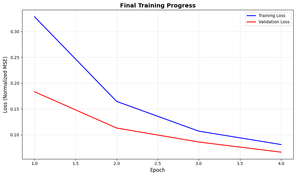
Step 7: Training Summary#
Training is complete! The plots above were updated in real-time during training. Let’s review the final training statistics and create a clean summary figure.
[ ]:
# Close previous figures and create final summary figure
plt.close("all")

history = results["history"]
epochs = range(1, len(history["train_loss"]) + 1)

# Create final summary figure
fig, ax = plt.subplots(figsize=(10, 6))

# Plot training and validation loss
ax.plot(epochs, history["train_loss"], "b-", label="Training Loss", linewidth=2)
ax.plot(epochs, history["val_loss"], "r-", label="Validation Loss", linewidth=2)
ax.set_xlabel("Epoch", fontsize=12)
ax.set_ylabel("Loss (Normalized MSE)", fontsize=12)
ax.set_title("Final Training Progress", fontsize=14, fontweight="bold")
ax.legend(fontsize=10)
ax.grid(visible=True, alpha=0.3)

plt.tight_layout()
plt.show()

# Print training summary
print("\n" + "=" * 80)
print("TRAINING SUMMARY")
print("=" * 80)
print(f"Total Epochs: {len(history['train_loss'])}")
print(f"\nInitial Validation Loss: {history['val_loss'][0]:.6f}")
print(f"Final Training Loss: {history['train_loss'][-1]:.6f}")
print(f"Final Validation Loss: {history['val_loss'][-1]:.6f}")
print(f"Best Validation Loss: {results['best_val_loss']:.6f} (Epoch {results['best_epoch']})")
print(f"\nImprovement: {(1 - history['val_loss'][-1] / history['val_loss'][0]) * 100:.1f}%")
print("=" * 80)
print("✅ Step 7 complete: Training summary generated")
================================================================================
TRAINING SUMMARY
================================================================================
Total Epochs: 4

Initial Validation Loss: 0.183471
Final Training Loss: 0.081217
Final Validation Loss: 0.066449
Best Validation Loss: 0.066449 (Epoch 4)

Improvement: 63.8%
================================================================================
✅ Step 7 complete: Training summary generated
Step 8: Summary and Next Steps#
Summary:
In this tutorial, we:
Generated a CDL channel training dataset using Sionna
Configured and trained an AI channel filter
Saved the trained model for use in channel estimation
Model Location:
Checkpoints: /opt/nvidia/aerial-framework/out/ai_tukey_filter_tutorial_training/checkpoints
Configuration: {results[‘checkpoint_dir’]}/model_config.yaml
Next Steps:
Try out the trained model in the PUSCH Channel Filter Lowering Tutorial.
Experiment with different AI models: Try different model architectures, learning rates, or dataset sizes to improve performance.
Performance Tips:
Larger datasets (65K+ samples) typically improve generalization
Training on diverse channel conditions (speed, delay spread) helps robustness
Monitor validation loss to detect overfitting