2. Reference PUSCH Receiver

A step-by-step PUSCH receiver walkthrough that:

• loads pipeline input data from a test vector (TV)

• calls each block individually

• shows plots along the way

Prerequisites: uv (already installed inside container)

Time: ~5-10 minutes

The pipeline is divided into two parts:

• (Steps 3-8) PUSCH Inner Receiver pipeline blocks: Channel Estimation, Equalization and Soft Demapping.

• (Steps 9-10) PUSCH Outer Receiver blocks: Descramble, Derate, LDPC decoding, and CRC.

Step 1: Import Dependencies

Import the required packages from the RAN Python environment. These were installed when the docs environment was set up via CMake.

import sys

from tutorial_utils import get_project_root, is_running_in_docker

# Ensure running inside Docker container
if not is_running_in_docker():
    print("\n❌ This notebook must be run inside the Docker container.")
    print(
        "\nPlease refer to the User Guide for instructions on running "
        "tutorial notebooks in the Docker container."
    )
    sys.exit(1)

PROJECT_ROOT = get_project_root()

# Path to ran python package: aerial-framework/ran/py
ran_py_path = PROJECT_ROOT / "ran" / "py"

print("✅ RAN package is available from docs environment")
print("✅ Step 1 complete: Dependencies imported")

Step 2: Import & Load Test Vector Data

The default TV contains everything needed to run the pipeline blocks as in the tests. The data inside the TV was obtained from NVIDIA Aerial 5GModel, a MATLAB implementation of 5G PHY layer, functionally matching MATLAB’s 5G Toolbox.

from pprint import pprint

import matplotlib.pyplot as plt
import numpy as np

from ran.constants import SC_PER_PRB
from ran.phy.numpy import pusch
from ran.utils import hdf5_load

tv_dir = ran_py_path.parent / "test_data"
tv_name = "TVnr_7204_cuPHY_simple.h5"
tv_path = tv_dir / tv_name

# Load PUSCH Inputs (dictionary)
inputs = hdf5_load(tv_path)
with np.printoptions(edgeitems=2):  # show 2 items at the start/end of each dimension
    pprint(inputs)
print("✅ Step 2 complete: Test vector data loaded")

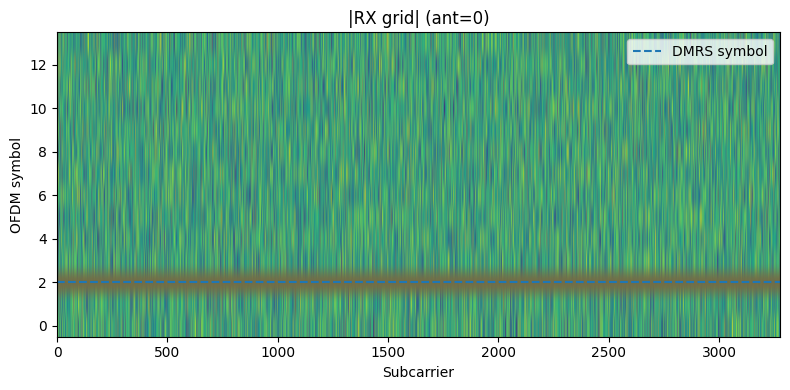
Step 3: RE Demapping

The first operation is extracting the Data and the Demodulation Reference Signal (DMRS) REs.

# Split RX grid into PRB band and DMRS/DATA symbol sets
rx_grid = inputs["xtf"]  # (n_f, n_t, n_ant)
n_f_start = SC_PER_PRB * inputs["start_prb"]
n_f_end = n_f_start + SC_PER_PRB * inputs["n_prb"]
freq_slice = slice(n_f_start, n_f_end)

dmrs_sym = rx_grid[freq_slice, inputs["sym_idx_dmrs"], :]  # (nf, n_dmrs, n_ant)
data_sym = rx_grid[freq_slice, inputs["sym_idx_data"], :]  # (nf, n_data, n_ant)
print("✅ Step 3 complete: RE demapping finished")

# Plot RX grid (ant=0)
nf, nt, nant = rx_grid.shape
plt.figure(figsize=(8, 4))
plt.imshow(np.abs(rx_grid[:, :, 0]).T, aspect="auto", origin="lower")
plt.title("|RX grid| (ant=0)")
plt.xlabel("Subcarrier")
plt.ylabel("OFDM symbol")

# Overlay DMRS and DATA symbol indices
for s in np.atleast_1d(inputs["sym_idx_dmrs"]):
    plt.axhline(y=s, linestyle="--", label="DMRS symbol")
plt.legend()
plt.tight_layout()
plt.show()

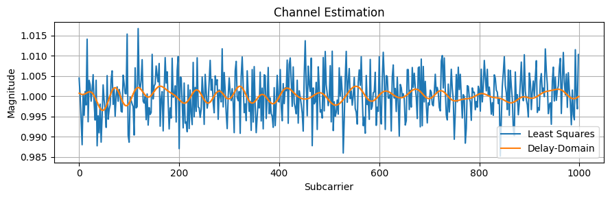
Step 4: DMRS Generation, Extraction & Channel Estimation

Next, we generate the DMRS symbols that were sent by the transmitter (x_dmrs), and extract the received DMRS symbols from the RX grid REs (y_dmrs). Using x_dmrs and y_dmrs, we can estimate the channel (h_est).

# DMRS symbol generation (gold sequence + QPSK mapping)
r_dmrs, _ = pusch.gen_dmrs_sym(
    slot_number=inputs["slot_number"],
    n_f=rx_grid.shape[0],
    n_dmrs_id=inputs["n_dmrs_id"],
    sym_idx_dmrs=inputs["sym_idx_dmrs"],
)

# Compute Transmitted DMRS (Symbols -> Orthogonal Cover Codes -> Scrambling)
x_dmrs = pusch.embed_dmrs_ul(
    r_dmrs=r_dmrs,
    nl=inputs["nl"],
    port_idx=inputs["port_idx"],
    vec_scid=inputs["vec_scid"],
    energy=inputs["energy"],
)
# Extract Received DMRS REs from RX grid
y_dmrs = pusch.extract_raw_dmrs_type_1(
    xtf_band_dmrs=dmrs_sym,
    nl=inputs["nl"],
    port_idx=inputs["port_idx"],
)

# Least Squares Channel Estimation
h_est_ls = pusch.channel_est_ls(x_dmrs=x_dmrs / 2, y_dmrs=y_dmrs)  # (6*n_prb, n_layers, n_ant)

# Delay-domain Channel Estimation (w/ truncation + interpolation)
h_est = pusch.channel_est_dd(
    x_dmrs=x_dmrs / 2, y_dmrs=y_dmrs
)  # (12*n_prb, n_layers, n_ant, n_dmrs)

# Plot Channel Estimation Comparison
plt.figure(figsize=(9, 3))
n_sc = 1000  # number of subcarriers to plot
x = np.arange(n_sc)
h = h_est[:n_sc, 0, 0, 0]  # single layer, single antenna, single dmrs symbol
h_ls = h_est_ls[: n_sc // 2, 0, 0]  # LS only on even subcarriers
plt.plot(x[::2], np.abs(h_ls), label="LS")
plt.plot(x, np.abs(h), label="DD")
plt.title("Channel Estimation")
plt.xlabel("Subcarrier")
plt.ylabel("Magnitude")
plt.legend(["Least Squares", "Delay-Domain"])
plt.tight_layout()
plt.grid()
plt.show()
print("✅ Step 4 complete: DMRS generation and channel estimation finished")

Step 5: Noise/Interference Covariance Estimation

Next, we need to estimate the contribution of noise and interference in the received signal to perform the MMSE-IRC equalization in the next step. We compute the covariance matrix of the noise and interference (n_cov).

n_cov, mean_noise_var = pusch.estimate_covariance(
    xtf_band_dmrs=dmrs_sym,
    x_dmrs=x_dmrs,
    h_est_band_dmrs=h_est,
    rww_regularizer_val=inputs["rww_regularizer_val"],
)  # (n_ant, n_ant, n_prb, n_pos)
print("✅ Step 5 complete: Noise/interference covariance estimated")

Step 6: Pre-equalization Metrics: Noise, RSRP, SINR, RSSI

Using the estimated channel and covariance, we can estimate the noise variance, RSRP, and SINR.

# Measure RSSI based on DMRS REs
dmrs_rssi_db, dmrs_rssi_reported_db = pusch.measure_rssi(xtf_band_dmrs=dmrs_sym)

# Estimate Noise, RSRP, SINR
noise_db, rsrp_db, sinr_db = pusch.noise_rsrp_sinr_db(
    mean_noise_var=mean_noise_var,
    h_est=h_est,
    layer2ue=inputs["layer2ue"],
    n_ue=inputs["n_ue"],
)
print("✅ Step 6 complete: Pre-equalization metrics computed")

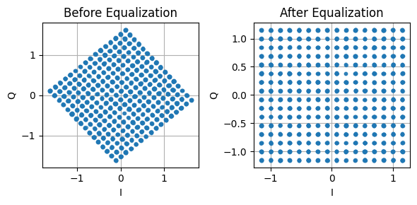
Step 7: Equalization and Post-Equalization Metrics

Now, the data symbols (data_sym) are equalized using the estimated channel (h_est) and the noise/interference covariance (n_cov).

Additional metrics are computed after equalization, like the post-equalization noise variance and SINR. These metrics can be useful for Layer 2 processing.

# 1) Equalization (MMSE-IRC)
x_est, ree = pusch.equalize(
    h_est=h_est,
    noise_intf_cov=n_cov,
    xtf_data=data_sym,
)

# 2) Post-Equalization Metrics (Noise, SINR)
post_noise_db, post_sinr_db = pusch.post_eq_noisevar_sinr(
    ree=ree,
    layer2ue=inputs["layer2ue"],
    n_ue=inputs["n_ue"],
)

# Plot Equalization Results (one antenna, one data symbol)
x_raw = data_sym[:, 0, 0]  # complex REs before equalization
x_eq = x_est[:, 0, 0]  # complex symbols after equalization
fig, axs = plt.subplots(1, 2, figsize=(6, 3), tight_layout=True)
axs[0].plot(x_raw.real, x_raw.imag, ".", alpha=0.5)
axs[0].set_title("Before Equalization")
axs[1].plot(x_eq.real, x_eq.imag, ".", alpha=0.5)
axs[1].set_title("After Equalization")
for a in axs:
    a.set_xlabel("I")
    a.set_ylabel("Q")
    a.grid()
print("✅ Step 7 complete: Equalization and post-equalization metrics computed")

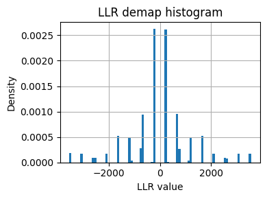
Step 8: Soft Demapping

Based on the equalized symbols (x_est), determine the log-likelihood ratios (LLRs) for each bit.

# Soft demap the equalized symbols to obtain the Log-Likelihood Ratios (LLRs)
llr_demap = pusch.soft_demapper(
    x=x_est,
    ree=ree,
    qam_bits=inputs["qam_bits"],
)  # (bits_per_sym, n_layer, n_tone, n_sym)

# Plot LLR histogram
plt.figure(figsize=(4, 3))
plt.hist(llr_demap.ravel(), bins=80, density=True)
plt.title("LLR demap histogram")
plt.xlabel("LLR value")
plt.ylabel("Density")
plt.tight_layout()
plt.grid()
plt.show()
print("✅ Step 8 complete: Soft demapping finished")

# Print intermediate checks
print("Intermediate checks:")
pprint(
    {
        "noiseVardB": noise_db,  # noise variance in dB
        "rsrpdB": rsrp_db,  # RSRP in dB
        "sinrdB": sinr_db,  # SINR in dB
        "postEqNoiseVardB": post_noise_db,  # post-equalization noise variance in dB
        "postEqSinrdB": post_sinr_db,  # post-equalization SINR in dB
        "dmrsRssiDb": dmrs_rssi_db,  # per-antenna RSSI in dB
        "dmrsRssiReportedDb": dmrs_rssi_reported_db,  # aggregated RSSI in dB
    }
)

Step 9: Outer receiver pipeline: Descramble, Derate, LDPC, CB concat, CRC

The remaining blocks handle the decoding of the transport block (TB) payload.

# Descramble the LLRs
llr_descr = pusch.descramble_bits(
    llrseq=llr_demap.ravel(order="F"),
    n_id=inputs["n_id"],
    n_rnti=inputs["n_rnti"],
)

# De-rate match the codeblocks
derate_cbs, nv_parity, derate_cbs_idxs, derate_cbs_sizes = pusch.derate_match(
    llr_descr=llr_descr,
    bgn=inputs["bgn"],
    c=inputs["c"],
    qam_bits=inputs["qam_bits"],
    k=inputs["k"],
    f=inputs["f"],
    k_prime=inputs["k_prime"],
    zc=inputs["zc"],
    nl=inputs["nl"],
    rv_idx=inputs["rv_idx"],
    nref=inputs["nref"],
    g=inputs["g"],
)

# LDPC decode the codeblocks
tb_cbs_est, num_itr = pusch.ldpc_decode(
    derate_cbs=derate_cbs,
    nv_parity=nv_parity,
    zc=inputs["zc"],
    c=inputs["c"],
    bgn=inputs["bgn"],
    i_ls=inputs["i_ls"],
    max_num_itr_cbs=inputs["max_num_itr_cbs"],
)

# Concatenate the codeblocks into a single transport block
tb_crc_est_vec, cb_err = pusch.codeblock_concatenation(
    tb_cbs_est=tb_cbs_est,
    c=inputs["c"],
    k_prime=inputs["k_prime"],
)

# CRC decode the complete transport block
tb_est, tb_err = pusch.crc_decode(tb_crc_est=tb_crc_est_vec)

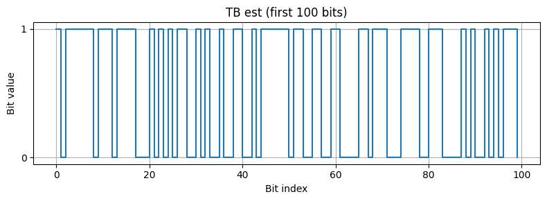
# Plot first n_bits bits of the payload (tb_est)
n_bits = 100
plt.figure(figsize=(8, 3))
plt.step(range(n_bits), tb_est[:n_bits], where="post")
plt.title(f"TB est (first {n_bits} bits)")
plt.xlabel("Bit index")
plt.ylabel("Bit value")
plt.yticks([0, 1])
plt.tight_layout()
plt.grid()
plt.show()
print("✅ Step 9 complete: Outer receiver pipeline finished")

# Print high-level outer receiver statistics
stats = {
    "num_codeblocks": int(inputs["c"]),
    "total_llr_bits": llr_demap.size,
    "avg_ldpc_iterations_per_cb": float(np.mean(num_itr)),
    "codeblock_crc_errors": int(np.sum(cb_err)),
    "tb_payload_bits": tb_est.size,  # payload + CRCs
    "tb_crc_bits": tb_crc_est_vec.size - tb_est.size,
    "tb_crc_errors": int(tb_err),
    "effective_code_rate": round(float(tb_est.size / llr_demap.size), 3),
    "avg_payload_bits_per_cb": round(float(tb_est.size / inputs["c"]), 3),
}

pprint(stats)

Step 10: Full receiver pipeline

The complete receiver pipeline can be run with a single call.

outputs = pusch.pusch_rx(inputs)  # full receiver pipeline (inner + outer)

# Validate full pipeline vs. step-by-step outputs
sinr_match = np.allclose(sinr_db, outputs["sinrdB"])
llr_match = np.allclose(llr_demap, outputs["LLR_demap"])
payload_match = np.allclose(tb_est, outputs["Tb_est"])
if sinr_match and llr_match and payload_match:
    print("✅ Full pipeline matches step-by-step results.")
print("✅ Step 10 complete: Full receiver pipeline verified")

Next Steps

Convert the inner receiver to JAX and compile it to a TRT engine. See next tutorial.

Explore

• NumPy pipeline: ran/py/src/ran/phy/numpy

• JAX pipeline: ran/py/src/ran/phy/jax

• Tutorials: docs/tutorials/

Troubleshooting

• Not running in Docker? This notebook must be run inside the Docker container. See the User Guide for instructions on running tutorial notebooks in the Docker container.

• RAN package import fails? Ensure the docs Python environment is set up: uv run ./scripts/setup_python_env.py setup docs --extras dev ran_mlir_trt (or ran_base if MLIR-TRT is disabled)

• Missing ipynb notebook? Run uv run ./scripts/setup_python_env.py jupytext_convert docs to convert the notebooks to ipynb files. Execute from the top-level aerial-framework directory. The notebook files are generated in docs/tutorials/generated/.

• Cannot serve notebook? Run uv run jupyter-lab --notebook-dir=docs/tutorials/generated to serve the notebooks. Execute from the top-level aerial-framework directory. The link to jupyterlab is displayed in the terminal.