Calculate and Plot the Distribution of Phonemes in a TTS Dataset#

In this tutorial, we will analyze the phonemes distribution of a ljspeech text corpus with a reference text corpus. The reference corpus is assumed to have the right phoneme distribution.

Our analysis will comprise creating a bar graph of both reference and sample phoneme distribution. Secondly, we will also calculate the difference in ljspeech phoneme distribution compared to a reference distribution.

Install all the required packages.

!pip install bokeh cmudict prettytable nemo_toolkit['all']
!pip install protobuf==3.20.0

# Put all the imports here for ease of use, and cleanliness of code 
import os
import pprint
import json
# import nemo g2p class for grapheme to phoneme
from nemo_text_processing.g2p.modules import EnglishG2p

# Bokeh
from bokeh.io import output_notebook, show
from bokeh.plotting import figure, output_file, show
from bokeh.io import curdoc, export_png
from bokeh.models import NumeralTickFormatter
output_notebook()

from prettytable import PrettyTable

# Counter 
import collections
from collections import Counter

pp = pprint.PrettyPrinter(indent =4, depth=10)

Get arpabet file#

Get the CMU grapheme to phoneme dictionary from nemo.

!wget https://raw.githubusercontent.com/NVIDIA/NeMo/v1.12.0/scripts/tts_dataset_files/cmudict-0.7b_nv22.08

Create the g2p object. This object will be used throughout to convert grapheme to phoneme

g2p = EnglishG2p(phoneme_dict="cmudict-0.7b_nv22.08", ignore_ambiguous_words=False)

Reference distribution:#

We will use a reference distribution that not only covers every phoneme in the English language (there are 44) but also exhibits the same frequency distribution as English. We can therefore use this reference distribution to compare the phoneme distribution of other datasets. This enables the identification of gaps in data, such as the need for more samples with a particular phoneme.

We will use NeMo grapheme to phoneme to convert words to phonemes.
List all the phonemes in g2p dict

# create a list of the CMU phoneme symbols
phonemes = {k: v[0] for k, v in g2p.phoneme_dict.items()}
pp.pprint(list(g2p.phoneme_dict.items()))

Load reference distribution#

We will load the reference freq distribution and visualize them in this section.

ref_corpus_file = "text_files/phoneme-dist/reference_corpus.json"
with open(ref_corpus_file) as f:
    freqs_ref = json.load(f)

Lets take a peek into the reference distribution

freqs_ref =dict(sorted(freqs_ref.items()))

xdata_ref = list(freqs_ref.keys())
ydata_ref = list(freqs_ref.values())

pp.pprint(freqs_ref)

Plot the reference frequency distribution

p = figure(x_range=xdata_ref, y_range=(0, 5000), plot_height=300, plot_width=1200, title="Reference phoneme frequency distribution",toolbar_location=None, tools="")

curdoc().theme = 'dark_minimal'

# Render and show the vbar plot
p.vbar(x=xdata_ref, top=ydata_ref)

# axis titles 
p.xaxis.axis_label = "Arpabet phonemes"
p.yaxis.axis_label = "Frequency of occurrence"

# display adjustments 
p.title.text_font_size = '20px'
p.xaxis.axis_label_text_font_size = '18px'
p.yaxis.axis_label_text_font_size = '18px'
p.xaxis.major_label_text_font_size = '6px'
p.yaxis.major_label_text_font_size = '18px'

show(p)

Now write a function to get the word frequencies of a text corpus.

def get_word_freq(filename):
    """
        Function to find phoneme frequency of a corpus.
        arg: filename: Text corpus filepath.
        return: frequencies of every phoneme in the file.
    """
    freqs = Counter()
    with open(filename) as f: 
        for line in f: 
            for word in line.split(): 
                freqs.update(phonemes.get(word, [])) 
    return freqs

Sample corpus Phonemes#

We will take a look at the phoneme distribution of text from ljspeech dataset. We dont need the LJspeech wav files for this tutorial. Therefore for simplicity, we can use the Ljspeech transcripts file from text_files/phoneme-dist/Ljspeech_transcripts.csv

Remove wav filenames from Ljspeech_transcripts.csv to generate Ljspeech text corpus.

!awk -F"|" '{print $2}' text_files/phoneme-dist/Ljspeech_transcripts.csv > ljs_text_corpus.txt

Load the Ljspeech text corpus file and create a frequency distribution of the phonemes.
We will use NeMo grapheme to phoneme to convert words to cmu phonemes.

in_file_am_eng = 'ljs_text_corpus.txt'
freqs_ljs = get_word_freq(in_file_am_eng)

# display frequencies
freqs_ljs=dict(sorted(freqs_ljs.items()))

xdata_ljs = list(freqs_ljs.keys())
ydata_ljs = list(freqs_ljs.values())

pp.pprint(freqs_ljs)

Lets plot the frequency distribution of ljspeech corpus like we did for reference distribution.

p = figure(x_range=xdata_ljs, y_range=(0, 70000), plot_height=300, plot_width=1200, title="Phoneme frequency distribution of ljspeech corpus",toolbar_location=None, tools="")

curdoc().theme = 'dark_minimal'

# Render and show the vbar plot
p.vbar(x=xdata_ljs, top=ydata_ljs)

# axis titles 
p.xaxis.axis_label = "Arpabet phonemes"
p.yaxis.axis_label = "Frequency of occurrence"

# display adjustments 
p.title.text_font_size = '20px'
p.xaxis.axis_label_text_font_size = '18px'
p.yaxis.axis_label_text_font_size = '18px'
p.xaxis.major_label_text_font_size = '6px'
p.yaxis.major_label_text_font_size = '18px'

show(p)

Plot distribution together#

we will need a canonical list of the CMU dict symbols and need to know what the length of that is compared to our corpus.

CMU phones:  
['AA0', 'AA1', 'AA2', 'AE0', 'AE1', 'AE2', 'AH0', 'AH1', 'AH2', 'AO0', 'AO1', 'AO2', 'AW0', 'AW1', 'AW2', 'AY0', 'AY1', 'AY2', 'B', 'CH', 'D', 'DH', 'EH0', 'EH1', 'EH2', 'ER0', 'ER1', 'ER2', 'EY0', 'EY1', 'EY2', 'F', 'G', 'HH', 'IH0', 'IH1', 'IH2', 'IY0', 'IY1', 'IY2', 'JH', 'K', 'L', 'M', 'N', 'NG', 'OW0', 'OW1', 'OW2', 'OY0', 'OY1', 'OY2', 'P', 'R', 'S', 'SH', 'T', 'TH', 'UH0', 'UH1', 'UH2', 'UW0', 'UW1', 'UW2', 'V', 'W', 'Y', 'Z', 'ZH']

arpa_list = g2p.phoneme_dict.values()
cmu_symbols = set()
for pronunciations in arpa_list:
    for pronunciation in pronunciations:
        for arpa in pronunciation:
            cmu_symbols.add(arpa)
cmu_symbols = list(cmu_symbols)
cmu_symbols.sort()
print(cmu_symbols)

Combine two distribution together.

data_combined = dict.fromkeys(cmu_symbols, 0)

for key in cmu_symbols: 
    if key in freqs_ref: 
        data_combined[key] += freqs_ref[key]
    if key in freqs_ljs: 
        data_combined[key] += freqs_ljs[key]

xdata_combined = list(data_combined.keys())
ydata_combined = list(data_combined.values())

pp.pprint(data_combined)

Phoneme comparison to a reference distribution#

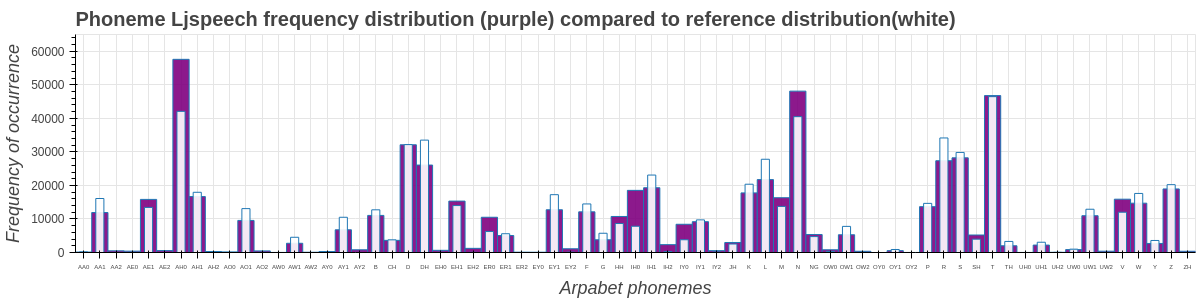
For analysis we will now look at the two distributions together.

First of all, we want to scale the reference distribution to the LJs distribution. Take the total phonemes in the Ljspeech distribution and total reference distribution phonemes and calculate a scaling factor then scale the reference distribution phoneme volume to match the Ljspeech distribution and then plot the reference phoneme distribution against the Ljspeech phoneme distribution.

# get the total phonemes in the reference phonemes 
ref_total = sum(freqs_ref.values())

# get the total phonemes in the comparison dataset
ljs_ph_total = sum(freqs_ljs.values())

# The scale factor is: 
scale_ljs = ljs_ph_total / ref_total

scaled_for_ljs = {} 
for phonemes in freqs_ref.items(): 
    scaled_for_ljs[phonemes[0]] = int(phonemes[1] * scale_ljs)
    

xscaled_for_ljs = list(scaled_for_ljs.keys())
yscaled_for_ljs = list(scaled_for_ljs.values())

plot two distributions together

p = figure(x_range=xdata_combined, y_range=(0, 65000), plot_height=300, plot_width=1200, title="Phoneme Ljspeech frequency distribution (purple) compared to reference distribution(white)",toolbar_location=None, tools="")

curdoc().theme = 'dark_minimal'

# Render and show the vbar plot - this should be a plot of the comparison dataset
p.vbar(x=xdata_ljs, top=ydata_ljs, fill_alpha=0.9, fill_color='purple')

# Render a vbar plot to show the reference distribution
p.vbar(x=xscaled_for_ljs, top=yscaled_for_ljs, fill_alpha=0.9, fill_color='white', width=0.5)

# axis titles 
p.xaxis.axis_label = "Arpabet phonemes"
p.yaxis.axis_label = "Frequency of occurrence"

# display adjustments 
p.title.text_font_size = '20px'
p.xaxis.axis_label_text_font_size = '18px'
p.yaxis.axis_label_text_font_size = '18px'
p.xaxis.major_label_text_font_size = '6px'
p.yaxis.major_label_text_font_size = '12px'
p.yaxis.formatter = NumeralTickFormatter(format="0")

show(p)

Calculate key differences between reference distribution and total phonemes#

Here we will check the difference in volume and percentage between two corpus for each phoneme.

diff_combined = {} 
for phonemes in data_combined.items():
    if phonemes[0] in scaled_for_ljs : 
        difference = phonemes[1] - scaled_for_ljs[phonemes[0]]
        min_ = min(phonemes[1], scaled_for_ljs[phonemes[0]])
        max_ = max(phonemes[1], scaled_for_ljs[phonemes[0]])
        percentage = round(((1 - (min_ / max_)) * 100), 2)
        diff_combined[phonemes[0]] = (difference, percentage)       
    else : 
        diff_combined[phonemes[0]] = (0,0)

t = PrettyTable(['Phoneme', 'Difference in volume', 'Difference in percentage'])
for phonemes in diff_combined.items() : 
    t.add_row([phonemes[0], phonemes[1][0], phonemes[1][1]])
print(t)

Conclusion#

In this tutorial, we saw how to analyze the phoneme distribution of our data. We can look for any phonemes that need more representation in the dataset using the techniques explained in this tutorial. This tutorial should be followed up by balancing the phoneme distribution of the data. It can be achieved by adding more sentences that contain phonemes with less coverage.

NVIDIA Riva

Calculate and Plot the Distribution of Phonemes in a TTS Dataset

Contents