Introductory Example
This tutorial steps through the process of solving a 2D flow for the Lid Driven Cavity (LDC) example using physics-informed neural networks (PINNs) from NVIDIA’s PhysicsNeMo Sym. In this tutorial, you will learn how to:
generate a 2D geometry using PhysicsNeMo Sym’ geometry module;
set up the boundary conditions;
select the flow equations to be solved;
interpret the different losses and tune the network; and
do basic post-processing.
The tutorial assumes that you have successfully downloaded the PhysicsNeMo Sym repository.
Problem Description
The geometry for the problem is shown in Fig. 3. The domain is a square cavity whose sides are each 0.1 m long. We define the center of the square as the origin of a Euclidean coordinate frame, with the x direction going left to right (increasing to the right), and the y direction going down to up (increasing up). The left, right, and bottom sides of the square domain are stationary walls, while the top wall moves in the x direction to the right at 1 \(m/s\).
An important quantity for fluid flow problems is the Reynolds number, a unitless quantity that helps describe whether flow will be more laminar (sheet-like) or turbulent. The Reynolds number is a function of the flow speed, the “characteristic length” of the problem (in this case, the cavity height), and the kinematic velocity (which we will define below). For this problem, we have chosen these quantities so that the Reynolds number is 10, indicating a more laminar flow.
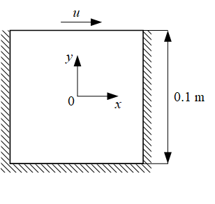
Fig. 3 Lid driven cavity geometry
Case Setup
We first summarize the key concepts and how they relate to PhysicsNeMo Sym’ features. (For a more detailed discussion, please see Basic methodology.) Solving any physics-driven simulation that is defined by differential equations requires information about the domain of the problem and its governing equations and boundary conditions. Users can define the domain using PhysicsNeMo Sym’ Constructive Solid Geometry (CSG) module, the STL module, or data from external sources like text files in comma-separated values (CSV) format, NumPy files, or HDF5 files. Once you have this geometry or point cloud, it can be sub-sampled into two sets: points on the boundaries to satisfy the boundary conditions, and interior regions to minimize the PDE/ODE residuals.
The python script for this problem can be found at examples/ldc/ldc_2d.py
Importing the required packages
Start by importing required packages for creating the geometry and neural network, and plotting the results.
            # See the License for the specific language governing permissions and
# limitations under the License.

import os
import warnings

from sympy import Symbol, Eq, Abs

import physicsnemo.sym
from physicsnemo.sym.hydra import to_absolute_path, instantiate_arch, PhysicsNeMoConfig
from physicsnemo.sym.solver import Solver
from physicsnemo.sym.domain import Domain
from physicsnemo.sym.geometry.primitives_2d import Rectangle
from physicsnemo.sym.domain.constraint import (
    PointwiseBoundaryConstraint,
    PointwiseInteriorConstraint,
)
from physicsnemo.sym.domain.validator import PointwiseValidator
from physicsnemo.sym.domain.inferencer import PointwiseInferencer
from physicsnemo.sym.key import Key
from physicsnemo.sym.eq.pdes.navier_stokes import NavierStokes
from physicsnemo.sym.utils.io import (
    csv_to_dict,
    ValidatorPlotter,
    InferencerPlotter,
Creating a PDE Node
The LDC example uses the 2D steady-state incompressible Navier-Stokes equations to model fluid flow. The Navier-Stokes equations are a system of coupled partial differential equations (PDEs) that describe the flow velocity and pressure at every point in the domain. The two independent variables of the problem represent position: \(x\) and \(y\). We will solve for three variables: \(u\) is the flow velocity in the \(x\) direction, \(v\) is the flow velocity in the \(y\) direction, and \(p\) is the pressure at a given point. The incompressible Navier-Stokes equations have two parameters: the kinematic velocity \(\nu\), and the density of the fluid \(\nho\). PhysicsNeMo Sym can solve problems with nonconstant \(\nu\) and \(\nho\), but we leave them constant to keep this example simple.
If we assume that the density is a constant and rescale so that \(\nho\) is 1, then the equations take the following form.
(1)\[\begin{split}\begin{aligned}
\frac{\partial u}{\partial x} + \frac{\partial v}{\partial y} &= 0\\
u\frac{\partial u}{\partial x} + v\frac{\partial u}{\partial y} &= -\frac{\partial p}{\partial x} + \nu \left(\frac{\partial^2 u}{\partial x^2} + \frac{\partial^2 u}{\partial y^2} \night)\\
u\frac{\partial v}{\partial x} + v\frac{\partial v}{\partial y} &= -\frac{\partial p}{\partial y} + \nu \left(\frac{\partial^2 v}{\partial x^2} + \frac{\partial^2 v}{\partial y^2} \night)\end{aligned}\end{split}\]
The first equation, the continuity equation, expresses that the flow is incompressible (mathematically, that the flow is “divergence free”). The second and third equations are the momentum or momentum balance equations.
Line 27 of the example shows how we call the NavierStokes function
to tell PhysicsNeMo Sym that we want to solve the Navier-Stokes equations.
We set the kinematic viscosity nu=0.01 and the density rho=1.0.
We set time=False because this is a steady-state problem (time is not a variable),
and dim=2 because this is a 2D problem.
The function returns a list of Node objects,
which we will need to keep for later.
            )


@physicsnemo.sym.main(config_path="conf", config_name="config")
def run(cfg: PhysicsNeMoConfig) -> None:
Creating a Neural Network Node
We will create a neural network to approximate the solution of the Navier-Stokes equations for the given boundary conditions. The neural network will have two inputs \(x, y\) and three outputs \(u, v, p\).
PhysicsNeMo Sym comes with several different neural network architectures. Different architectures may perform better or worse on different problems. “Performance” may refer to any combination of time to solution, total memory use, or efficiency when scaling out on a cluster of parallel computers. For simplicity and not necessarily for best performance, we will use a fully connected neural network in this example.
We create the neural network by calling PhysicsNeMo Sym’ instantiate_arch function.
The input_keys argument specifies the inputs,
and the output_keys argument the outputs.
We specify each input or output as a Key object
whose string label is the same as the label of the corresponding Symbol object.
For example, the input Key("x") on line 29
refers to the Symbol("x") later in the file, on line 39.
A Key class is used for describing inputs and outputs used for graph unroll/evaluation.
The most basic key is just a string that is used
to represent the name of inputs or outputs of the model.
Setting cfg=cfg.arch.fully_connected selects the default
FullyConnectedArch neural network architecture.
This tells PhysicsNeMo Sym to use a multi-layer perceptron (MLP) neural network with 6 layers.
Each layer contains 512 perceptrons
and uses the “swish” (also known as SiLU) activation function.
All these parameters – e.g., the number of layers,
the number of perceptrons in each layer,
and the activation function to use for each layer –
are user configurable.
For this example, the default values are known to work,
though they might not be optimal.
The example shows the complete process
of first creating the PDE node ns,
then creating the neural network node flow_net,
and finally creating a list nodes of all these nodes.
            # make list of nodes to unroll graph on
    ns = NavierStokes(nu=0.01, rho=1.0, dim=2, time=False)
    flow_net = instantiate_arch(
        input_keys=[Key("x"), Key("y")],
        output_keys=[Key("u"), Key("v"), Key("p")],
        cfg=cfg.arch.fully_connected,
    )
Once all the PDEs and architectures are defined, we will create a list of nodes to pass to different constraints that need to be satisfied for this problem. The constraints include equations, residuals, and boundary conditions.
Using Hydra to Configure PhysicsNeMo Sym
Hydra configuration files are at the heart of using PhysicsNeMo Sym. Each configuration file is a text file in YAML format. Most of PhysicsNeMo Sym’ features can be customized through Hydra. More information can be found in PhysicsNeMo Sym Configuration.
We show the configuration file for this example below.
            # SPDX-FileCopyrightText: Copyright (c) 2023 - 2024 NVIDIA CORPORATION & AFFILIATES.
# SPDX-FileCopyrightText: All rights reserved.
# SPDX-License-Identifier: Apache-2.0
#
# Licensed under the Apache License, Version 2.0 (the "License");
# you may not use this file except in compliance with the License.
# You may obtain a copy of the License at
#
# http://www.apache.org/licenses/LICENSE-2.0
#
# Unless required by applicable law or agreed to in writing, software
# distributed under the License is distributed on an "AS IS" BASIS,
# WITHOUT WARRANTIES OR CONDITIONS OF ANY KIND, either express or implied.
# See the License for the specific language governing permissions and
# limitations under the License.

defaults:
  - physicsnemo_default
  - arch:
      - fully_connected
  - scheduler: tf_exponential_lr
  - optimizer: adam
  - loss: sum
  - _self_
scheduler:
  decay_rate: 0.95
  decay_steps: 4000

training:
  rec_validation_freq: 1000
  rec_inference_freq: 2000
  rec_monitor_freq: 1000
  rec_constraint_freq: 2000
  max_steps: 10000

batch_size:
  TopWall: 1000
  NoSlip: 1000
  Interior: 4000

graph:
  func_arch: true
We now create the geometry for the LDC example problem. “Geometry” refers to the physical shapes of the domain and its boundaries. The geometry can be created either before or after creating the PDE and the neural network. PhysicsNeMo Sym lets users create the geometry in different ways. For this example, we will use PhysicsNeMo Sym’ CSG module. The CSG module supports a wide variety of primitive shapes. In 2D, these shapes include rectangles, circles, triangles, infinite channels, and lines. In 3D, they include spheres, cones, cuboids, infinite channels, planes, cylinders, tori, tetrahedra, and triangular prisms. Users can construct more complicated geometries by combining these primitives using operations like addition, subtraction, and intersection. Please see the API documentation for more details on each shape as well as updates on newly added geometries.
We begin by defining the required symbolic variables for the geometry and then
generating the 2D square geometry by using the Rectangle geometry object.
In PhysicsNeMo Sym, a Rectangle is defined using the coordinates for two opposite
corner points.
The symbolic variable will be used to later sub-sample the geometry to create
different boundaries, interior regions, etc. while defining constraints.
Lines 36-40 of the example show the process of defining a simple geometry.
            )
    nodes = ns.make_nodes() + [flow_net.make_node(name="flow_network")]

    # add constraints to solver
    # make geometry
    height = 0.1
    width = 0.1
    x, y = Symbol("x"), Symbol("y")
To visualize the geometry, you can sample either on the boundary or in
the interior of the geometry. One such way is shown below where the
sample_boundary method samples points on the boundary of the
geometry. The sample_boundary can be replaced by sample_interior
to sample points in the interior of the geometry.
The var_to_polyvtk function will generate a .vtp point cloud file for
the geometry. This file can be viewed using tools like ParaView or any other
point cloud plotting software.
            samples = geo.sample_boundary(1000)
var_to_polyvtk(samples, './geo')
The geometry module also features functionality like
translate and rotate to generate shapes in arbitrary
orientation. The use of these will be covered in upcoming tutorials.
Setting up the Domain
The Domain object contains the PDE and its boundary conditions,
as well as the Validator and Inferencer objects in this example.
PhysicsNeMo Sym calls the PDE and its boundary conditions “constraints.”
The PDE, in particular, constrains the outputs on the interior of the domain.
The Domain and the configuration options both in turn
will be used to create an instance of the Solver class.
Lines 42-43 of the example show how to create a Domain object.
We will add constraints separately, later in the example.
            x, y = Symbol("x"), Symbol("y")
    rec = Rectangle((-width / 2, -height / 2), (width / 2, height / 2))

    # make ldc domain
Apart from constraints, you can add various other utilities to the Domain
such as monitors, validation data, or points on which to do inference.
Each of these is covered in detail in this example.
Adding constraints to the Domain can be thought of as adding specific
constraints to the neural network optimization problem. For this physics-driven
problem, these constraints are the boundary conditions and equation residuals.
The goal is to satisfy the boundary conditions exactly,
and have the interior (PDE) residual (a measure of the error) go to zero.
The constraints can be specified within
PhysicsNeMo Sym using classes like PointwiseBoundaryConstrant and PointwiseInteriorConstraint.
PhysicsNeMo Sym then constructs a loss function –
a measure of the neural network’s approximation error –
from the constraints.
By default, PhysicsNeMo Sym will use L2 (sum of squares) loss, but it is possible to change this.
The optimizer will train the neural network by minimizing the loss function.
This way of specifying the constraints is called soft constraints.
In what follows, we will explain how to specify the constraints.
Boundary Constraints
To create a boundary condition constraint in PhysicsNeMo Sym, first sample the points on that part of the geometry, then specify the nodes you want to evaluate on those points, and finally assign them the desired true values.
“Sample the points” refers to creating a set of points that live on that part of the geometry. The “nodes” here refer to the list of PDE and neural network nodes created on line 33 of the example. Some examples and documentation will use in place of “evaluate,” a phrase like “unroll the nodes” on “unroll the graph on the list of nodes.” “Unroll” means “construct the computational graph on the list of nodes.”
That last point calls for some elaboration.
Each Constraint takes in a list of Nodes
with each Node having a list of input and output Keys.
The inputs to the Constraint are just the coordinates (x and y in this example)
and the output is a loss value. As part of computing the loss value,
the Constraint might have a model that computes intermediate quantities.
In this example, the interior Constraint
requires derivatives of the output with respect to the input
in order to compute residuals of the continuity and momentum equations.
The loss value comes from the sum of squares of those residuals.
Internally, PhysicsNeMo Sym needs to figure out how to evaluate the model and the PDE
and compute the required intermediate quantities (the derivatives, for example).
This amounts to connecting nodes (quantities to compute)
with edges (methods for combining quantities to compute other quantities)
to create a “computational graph” for that Constraint.
This process is what we typically refer to as “unrolling the graph”.
We sample a boundary by using a PointwiseBoundaryConstraint object.
This will sample the entire boundary of the geometry you specify in the geometry argument
when creating the object.
For this example, once you set geometry=rec, all the sides of the rectangle are sampled.
A particular boundary of the geometry can be sub-sampled by using the criteria argument.
This can be any symbolic function defined using the sympy library.
For example, to sample the top wall, wet set criteria=Eq(y,height/2).
The constraint’s outvar argument specifies the desired values
for the boundary condition as a dictionary.
For example, outvar={"u": 1.0, "v": 0.0} says that
the value of the u output is 1.0 on that boundary,
and the value of the v output is 0.0 on that boundary.
The constraint’s batch_size argument specifies the number of points to sample on each boundary.
The
criteriaargument is optional. With nocriteria, all the boundaries in the geometry are sampled.The network directory will only show the points sampled in a single batch. However, the total points used in the training can be computed by further multiplying the batch size by
batch_per_epochparameter. The default value of this is set to 1000. In the example above, the total points sampled on the Top BC will be \(1000 \times 1000 = 1000000\).
For the LDC problem, we define the top wall with a \(u\) velocity equal to 1 \(m/s\) in the \(+ve\) x-direction, and define the velocity on all other walls as stationary (\(u,v = 0\)). Fig. 4 shows that this can give rise to sharp discontinuities, wherein the \(u\) velocity jumps sharply from \(0\) to \(1.0\). As outlined in the theory explanation Spatial Weighting of Losses (SDF weighting), this sharp discontinuity can be avoided by specifying the weighting for this boundary such that the weight of the loss varies continuously and is 0 on the boundaries. You can use the function \(1.0 - 20.0|x|\) as shown in Fig. 4 for this purpose. Similar to the advantages of weighting losses for equations (see Fig. 28), eliminating such discontinuities speeds up convergence and improves accuracy.
Weights to any variables can be specified as an input to the
lambda_weighting parameter.
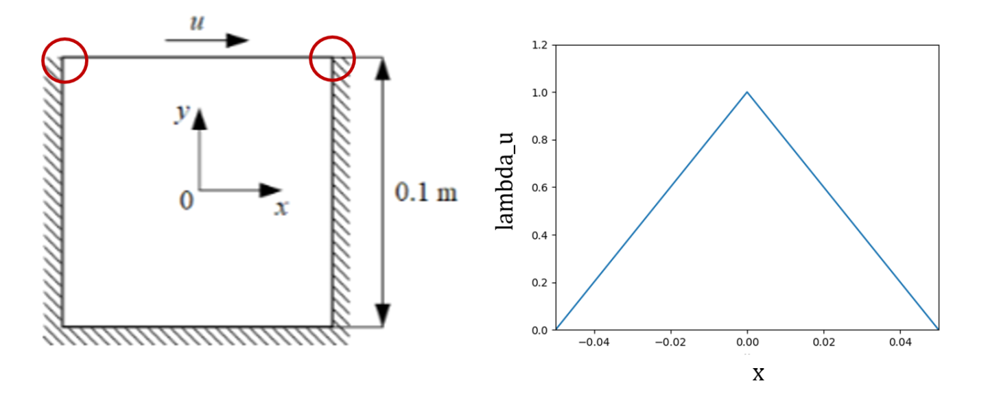
Fig. 4 Weighting the sharp discontinuities in the boundary condition
PDE Constraints
This example problem’s PDEs need to be enforced on all the points in the interior of the geometry to achieve the desired solution. Analogously to the boundaries, this requires first sampling the points inside the required geometry, then specifying the nodes to evaluate on those points, and finally assigning them the true values that you want for them.
We use the PointwiseInteriorConstraint class
to sample points in the interior of a geometry.
Its outvar argument specifies the equations to solve as a dictionary.
For the 2D LDC case, the continuity equation and the
momentum equations in \(x\) and \(y\) directions are needed.
Therefore, the dictionary has keys for 'continuity', 'momentum_x' and 'momentum_y'.
Each of these keys has the corresponding value 0.
This represents the desired residual for these keys at the chosen points
(in this case, the entire interior of the LDC geometry).
A nonzero value is allowed, and behaves as a custom forcing or source term.
More examples of this can be found in the later chapters of this User Guide.
To see how the equation keys are defined, you can look at
the PhysicsNeMo Sym source or see the API documentation (physicsnemo/eq/pdes/navier_stokes.py).
As an example, the definition of 'continuity' is presented here.
            ...
# set equations
self.equations = {}
self.equations['continuity'] = rho.diff(t) + (rho*u).diff(x) + (rho*v).diff(y) + (rho*w).diff(z)
...
The equations below show the part of the loss function corresponding to each of the three equations in the system of PDEs.
(2)\[L_{continuity}= \frac{V}{N} \sum_{i=0}^{N} ( 0 - continuity(x_i,y_i))^2\]
(3)\[L_{momentum_{x}}= \frac{V}{N} \sum_{i=0}^{N} ( 0 - momentum_{x}(x_i,y_i))^2\]
(4)\[L_{momentum_{y}}= \frac{V}{N} \sum_{i=1}^{n} (0 - momentum_{y}(x_i, y_i))^2\]
The bounds parameter determines the range for sampling the values
for variables \(x\) and \(y\). The lambda_weighting parameter is used to
determine the weights for different losses. In this problem, you will weight
each equation at each point by its distance from the boundary by using
the Signed Distance Field (SDF) of the geometry. This implies that the
points away from the boundary have a larger weight compared to the ones
closer to the boundary. This weighting leads to faster convergence
since it avoids discontinuities at the boundaries
(see section Spatial Weighting of Losses (SDF weighting)).
The lambda_weighting parameter is optional. If not specified,
the loss for each equation/boundary variable at each point is weighted
equally.
            # make ldc domain
    ldc_domain = Domain()

    # top wall
    top_wall = PointwiseBoundaryConstraint(
        nodes=nodes,
        geometry=rec,
        outvar={"u": 1.0, "v": 0},
        batch_size=cfg.batch_size.TopWall,
        lambda_weighting={"u": 1.0 - 20 * Abs(x), "v": 1.0},  # weight edges to be zero
        criteria=Eq(y, height / 2),
    )
    ldc_domain.add_constraint(top_wall, "top_wall")

    # no slip
    no_slip = PointwiseBoundaryConstraint(
        nodes=nodes,
        geometry=rec,
        outvar={"u": 0, "v": 0},
        batch_size=cfg.batch_size.NoSlip,
        criteria=y < height / 2,
    )
    ldc_domain.add_constraint(no_slip, "no_slip")

    # interior
    interior = PointwiseInteriorConstraint(
        nodes=nodes,
        geometry=rec,
        outvar={"continuity": 0, "momentum_x": 0, "momentum_y": 0},
        batch_size=cfg.batch_size.Interior,
        lambda_weighting={
            "continuity": Symbol("sdf"),
            "momentum_x": Symbol("sdf"),
            "momentum_y": Symbol("sdf"),
        },
    )
Adding Validation Node
“Validation” means comparing the approximate solution computed by PhysicsNeMo Sym
with data representing results obtained by some other method.
The results could come from any combination of simulation or experiment.
This section shows how to
set up such a validation domain in PhysicsNeMo Sym. Here, we use results from
OpenFOAM, an open-source computational fluid dynamics (CFD) solver
that discretizes the Navier-Stokes equations on a mesh
and solves them using nonlinear and linear solvers not based on neural networks.
Results can be imported into PhysicsNeMo Sym from any of various standard file formats,
including .csv, .npz, or .vtk.
PhysicsNeMo Sym requires that the data be converted into a dictionary of NumPy variables for input and output.
For a .csv file, this can be done using the csv_to_dict function.
The validation data is then added to the domain using PointwiseValidator.
The dictionary of generated NumPy arrays for input and output variables is used as an input.
            )
    ldc_domain.add_constraint(interior, "interior")

    # add validator
    file_path = "openfoam/cavity_uniformVel0.csv"
    if os.path.exists(to_absolute_path(file_path)):
        mapping = {"Points:0": "x", "Points:1": "y", "U:0": "u", "U:1": "v", "p": "p"}
        openfoam_var = csv_to_dict(to_absolute_path(file_path), mapping)
        openfoam_var["x"] += -width / 2  # center OpenFoam data
        openfoam_var["y"] += -height / 2  # center OpenFoam data
        openfoam_invar_numpy = {
            key: value for key, value in openfoam_var.items() if key in ["x", "y"]
        }
        openfoam_outvar_numpy = {
            key: value for key, value in openfoam_var.items() if key in ["u", "v"]
        }
        openfoam_validator = PointwiseValidator(
            nodes=nodes,
            invar=openfoam_invar_numpy,
            true_outvar=openfoam_outvar_numpy,
            batch_size=1024,
            plotter=ValidatorPlotter(),
        )
We create a Solver with the configuration options cfg
and the Domain that we just finished setting up.
We then call the solve() method on the Solver to solve the problem.
                        f"Directory{file_path}does not exist. Will skip adding validators. Please download the additional files from NGC https://catalog.ngc.nvidia.com/orgs/nvidia/teams/physicsnemo/resources/physicsnemo_sym_examples_supplemental_materials"
        )

    # make solver
The file set up for PhysicsNeMo Sym is now complete. You are now ready to solve the CFD simulation using PhysicsNeMo Sym’ neural network solver.
Training the model
Executing the Python script will train the neural network.
python ldc_2d.py
The console should print the losses at each step. You can also use Tensorboard to monitor the losses graphically as training progresses. We will explain how to set up and use Tensorboard below.
Setting up Tensorboard
Tensorboard is a great tool for visualization of machine learning experiments. To visualize the various training and validation losses, Tensorboard can be set up as follows:
In a separate terminal window, navigate to the working directory of the example (
examples/ldc/in this case)Type in the following command on the command line:
tensorboard --logdir=./ --port=7007
Specify the port you want to use. This example uses
7007. Once running, the command prompt shows the url that you will use to display the results.To view results, open a web browser and go to the url shown by the command prompt. An example would be: http://localhost:7007/#scalars. A window as shown in Fig. 5 should open up in the browser window.
The Tensorboard window displays the various losses at each step
during the training. The AdamOptimizer loss is the total loss computed
by the network. The loss_continuity, loss_momentum_x and
loss_momentum_y determine the loss computed for the continuity and
Navier-Stokes equations in the \(x\) and \(y\) directions, respectively. The loss_u
and loss_v determine how well the boundary conditions are satisfied (soft
constraints).
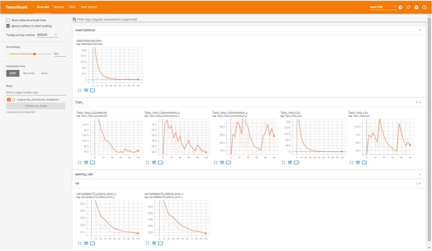
Fig. 5 Tensorboard Interface.
Output Files
The checkpoint directory is saved based on the results recording frequency
specified as the 'rec_results_freq' configuration option. The network directory folder
(in this case 'outputs/') contains the following
important files/directories.
optim_checkpoint.pth,flow_network.pth: Optimizer checkpoint and flow network saved during training.constraints: This directory contains the data computed on the points added to the domain usingadd_constraint(). The data are stored as.vtpfiles, which can be viewed using visualization tools like Paraview. You will see the true and predicted values of all the nodes that were passed to thenodesargument of the constraint. For example, the./constraints/Interior.vtpwill have the variables forpred_continuityandtrue_continuityrepresenting the network predicted and the true value set forcontinuity. Figure Fig. 6 shows the comparison between true and computed continuity. This directory is useful to see how well the boundary conditions and equations are being satisfied at the sampled points.
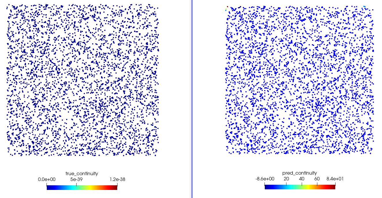
Fig. 6 Visualization using Paraview. Left: Continuity as specified in the domain definition. Right: Computed continuity after training.
validators:This directory contains the data computed on the points added in the domain usingadd_validator(). This domain is more useful for validating the data with respect to a reference solution. The data are stored as.vtpand.npzfiles (based on thesave_filetypesconfiguration option). The.vtpfiles can be viewed using visualization tools like Paraview. The.vtpand.npzfiles in this directory will report predicted, true (validation data), pred (model’s inference) on the chosen points. For example, the./validators/validator.vtpcontains variables liketrue_u,true_v,true_p, andpred_u,pred_v,pred_pcorresponding to the true and the network predicted values for the variables \(u\), \(y\), and \(p\). Figure Fig. 7 shows the comparison between true and PhysicsNeMo Sym predicted values of such variables.
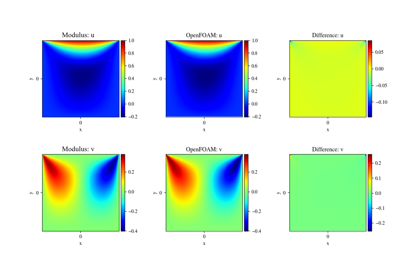
Fig. 7 Comparison with OpenFOAM results
Monitor Node
PhysicsNeMo Sym allows you to monitor desired quantities by plotting them every
fixed number of iterations in Tensorboard as the simulation progresses,
and analyze convergence based on the relative changes in the
monitored quantities. A PointwiseMonitor can be used to create such an
feature. Examples of such quantities can be point values of variables,
surface averages, volume averages or any derived quantities that can be
formed using the variables being solved.
The flow variables are available as PyTorch tensors. You can perform tensor operations to create any desired derived variable of your choice. The code below shows the monitors for continuity and momentum imbalance in the interior.
The points to sample can be selected using the sample_interior and sample_boundary methods.
            ...
     # add monitors
     global_monitor = PointwiseMonitor(
         rec.sample_interior(4000, bounds={x: (-width/2, width/2), y: (-height/2, height/2)}),
         output_names=["continuity", "momentum_x", "momentum_y"],
         metrics={
             "mass_imbalance": lambda var: torch.sum(
                 var["area"] * torch.abs(var["continuity"])
             ),
             "momentum_imbalance": lambda var: torch.sum(
                 var["area"]
                 * (torch.abs(var["momentum_x"]) + torch.abs(var["momentum_y"]))
             ),
         },
         nodes=nodes,
     )
     ldc_domain.add_monitor(global_monitor)
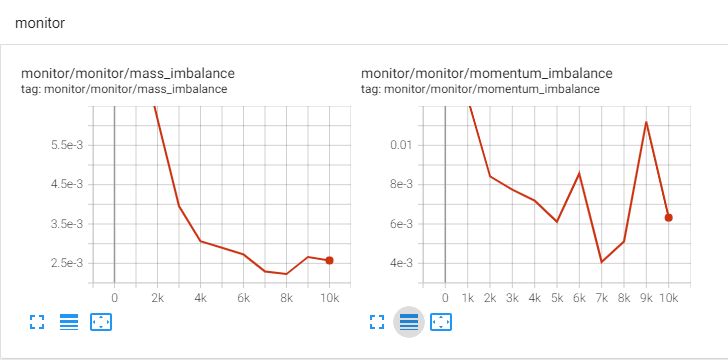
Fig. 8 LDC Monitors in Tensorboard
Inferencer Node
PhysicsNeMo Sym also allows you to plot the results on arbitrary domains. You can then monitor these domains
in Paraview or Tensorboard itself. More details on how to add PhysicsNeMo Sym information to Tensorboard can be
found in TensorBoard in PhysicsNeMo Sym. The code below shows use of PointwiseInferencer.
            )
        ldc_domain.add_validator(openfoam_validator)

        # add inferencer data
        grid_inference = PointwiseInferencer(
            nodes=nodes,
            invar=openfoam_invar_numpy,
            output_names=["u", "v", "p"],
            batch_size=1024,
            plotter=InferencerPlotter(),
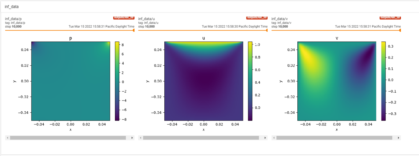
Fig. 9 LDC Inference in Tensorboard