

User Guide#
Information on all views, controls, and workflows within the tool.
Overview#
Nsight Deep Learning Designer is a software tool whose goal is to speed up Deep Learning developers’ workflow by providing tools to design and profile models in an interactive manner.
Using Nsight Deep Learning Designer, you can iterate faster on your model by rapidly launching inference runs and profiling the layers’ behavior using GPU performance counters.
Nsight Deep Learning Designer is available as a desktop application for Windows, Linux, and macOS (host only). It is also available as a Nsight Cloud container that can be hosted on a server and accessed through a browser.
Nsight Deep Learning Designer supports two native model formats:
XDL - Nsight Deep Learning Designer’s extensible deep-learning format. XDL is Nsight Deep Learning Designer’s bridge for bringing PyTorch models to DLD: it maps closely to PyTorch in both level of abstraction and round-trip fidelity, allowing models to be imported from and exported back to PyTorch. XDL is XML-based and adds higher-level abstractions such as reusable templates and formula-based operator parameters that are well suited to interactive authoring on the canvas. See the XDL Format chapter for details.
ONNX - the Open Neural Network Exchange format. ONNX models can be opened, edited, and saved directly, and are the format used for deployment and profiling.
Both formats can be opened and edited side by side. XDL models are converted to ONNX for inference operations. Profiling uses TensorRT and ONNX Runtime as companion inference frameworks.
Model Design#
Understanding how to efficiently design a model inside Nsight Deep Learning Designer and leverage the various features to do so is crucial. The workflows in this chapter apply to both ONNX and XDL models unless otherwise noted. Some tool windows and actions are only available for ONNX or XDL models; see relevant sections for details.
Creating a New Model#
Nsight Deep Learning Designer can both open an existing model and create a new one from scratch.
ONNX#
To create a new ONNX model, use File > New File and select ONNX to open the dedicated wizard.
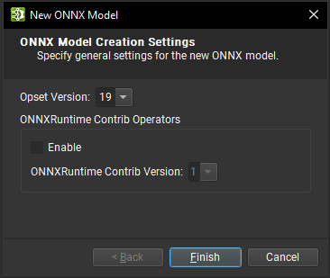
The wizard lets you pick the ONNX Opset version for the new model. All Opsets from version 1 up to and including version 23 are supported. Importing the ONNXRuntime Contrib Operator set makes the additional operators recognized by ONNX Runtime available on the canvas.
XDL#
To create a new XDL model, use File > New File and select XDL. This will open a blank canvas for a new XDL document. See the PyTorch Importer chapter on how to import an existing PyTorch model into Nsight Deep Learning Designer and convert it to XDL.
Workspace#
Each opened model is represented by a document tab in the Nsight Deep Learning Designer workspace. Multiple models can be opened simultaneously and arranged using the docking system; ONNX and XDL documents share the same workspace. The central element in the Nsight Deep Learning Designer workspace is the canvas where you create and edit your model graph by dropping layer nodes and creating connections between them. The workspace can be arranged using the dockable tool windows to best fit your desired workflow. All tool windows can be found under View > Windows and the model canvas context menu. Refer to the commands under the Window menu to save, apply or reset layouts.
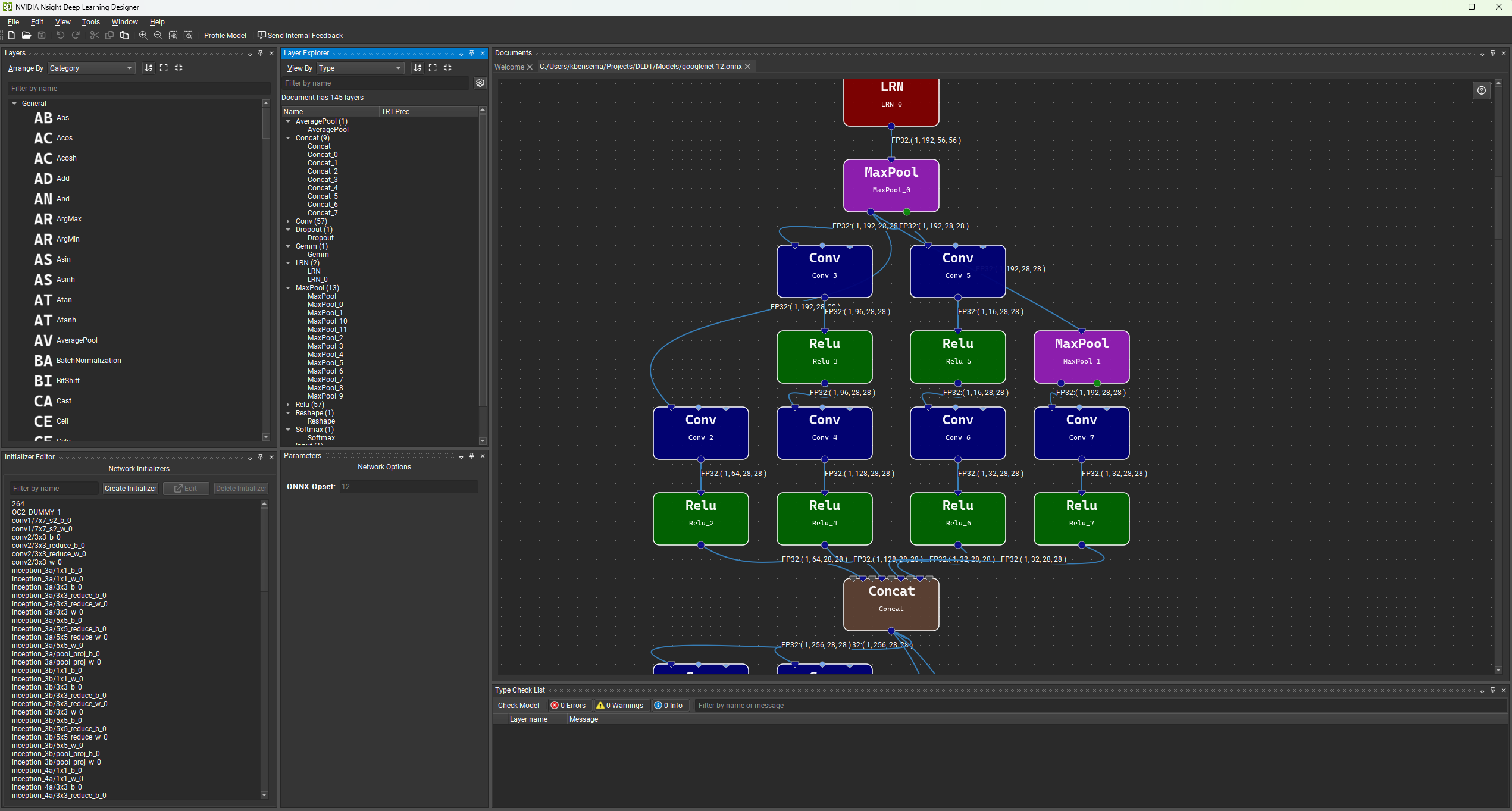
The default workspace is composed of the Layer Palette, the Parameter Window, Layer Explorer and the Type Checking window.
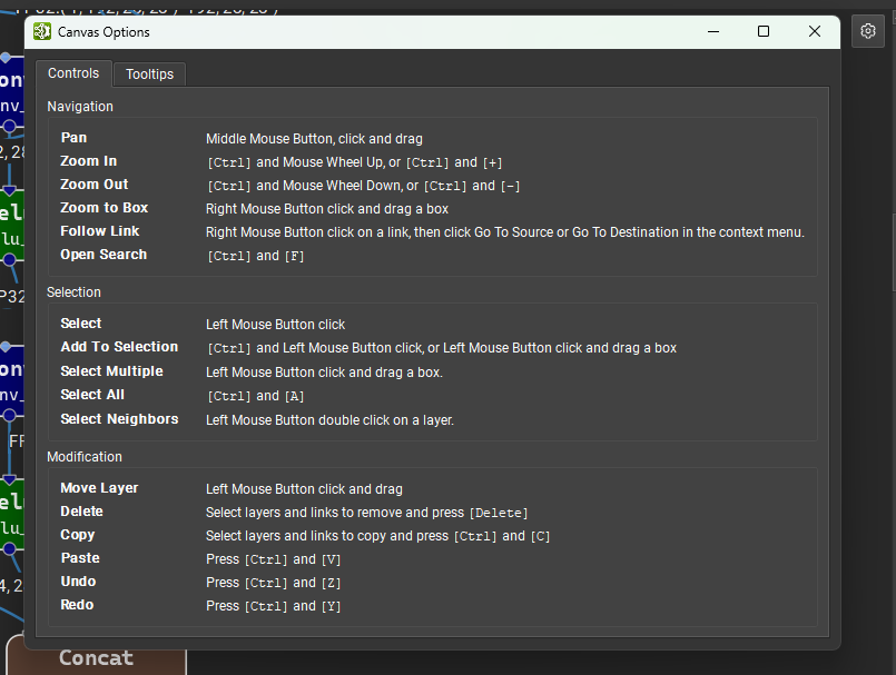
When first loading a model, the canvas will show the entire model graph. The user can zoom in and out with Ctrl + Mouse Wheel, or can zoom to a region by right clicking and dragging a box. Scrolling with the mouse wheel pans the view up and down, and clicking and dragging with the middle mouse button pans the view in any direction. A complete list of navigation actions may be viewed by clicking the Model Canvas Options button (gear icon) in the top-right corner of the canvas and selecting the Controls tab.
To make it easier to align nodes visually in the canvas a background grid can be enabled using the View > Show Grid menu action. Nodes in the canvas may be identified by their unique name (automatically generated by Nsight Deep Learning Designer if missing) and by their layer type.
Editing actions that modify the current graph or model will mark the document as modified. Changes are only reflected on disk once the model is saved using the File > Save menu action or the Ctrl + S shortcut. Editing actions from the current session can be undone and redone, using the Edit > Undo/Redo menu actions or the respective Ctrl + Z and Ctrl + Y shortcuts.
Layout#
The first time a model is opened in Nsight Deep Learning Designer, a layout algorithm automatically positions the nodes on the canvas. Node positions are persisted with the model so they can be restored on re-open. The layout algorithm can be run explicitly on any model using the View > Arrange Nodes menu action.
Colors#
Nodes in the canvas are colored according to their type. As there are too many node types for each one to receive a distinguishable unique color, related node types share the same color. Certain classes of nodes also have different shapes: input and output nodes are represented as diamonds, while composite nodes such as local functions, XDL templates, or nodes containing subgraphs are represented as sharp-cornered rectangles rather than rounded rectangles.
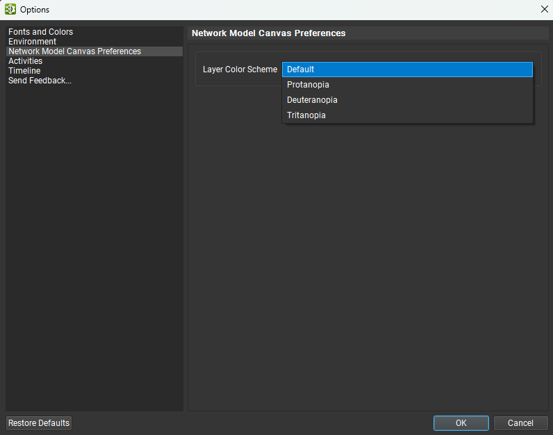
Nsight Deep Learning Designer provides some alternative color schemes, which may be helpful for individuals with color vision deficiency. The color scheme can be changed from the Network Canvas Preferences page of the Options (Tools > Options) dialog. The figure below shows the available color schemes.
Search Bar#
As a model can contain a large number of nodes, search functionality is present in Nsight Deep Learning Designer to make it easier to find specific nodes in the canvas. The search bar is accessible either by using the Ctrl + F shortcut in the canvas or through the Edit > Search Layer menu action. You may search by node name or type — the dropdown next to the text box controls the search criterion. The controls in the search bar allow to cycle between the next and previous match, when cycling the view focuses on the current matched node. Note that the text search is case-sensitive.
Exporting the Canvas#
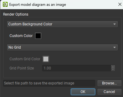
The entire model canvas may be exported to a single image file using the File > Export > Export Canvas As Image menu action. The background color, grid color and presence, and image save location may be set from the dialog pictured below. The supported image formats are PNG, JPEG, and SVG.
Layers#
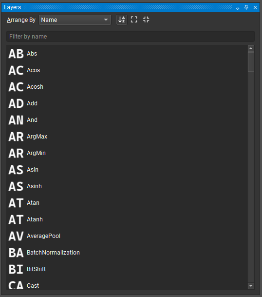
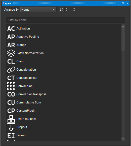
The Layer Palette holds the list of available operators that can be added to the current model. For ONNX models, the palette is populated from the operator sets the model imports; for XDL models, the palette lists the XDL operator library. Layers can be arranged by name, collection, or category. The Layer Palette can also be sorted or filtered. To add new layer instances to the canvas, simply drag and drop from the palette.
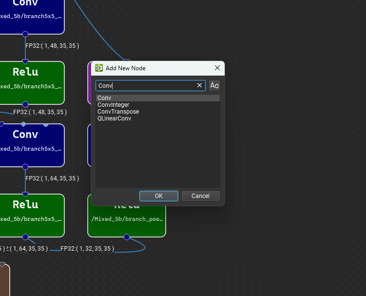
Alternatively, place the mouse cursor anywhere in the model canvas and press ‘Control + Space’ to open a quick node add dialog, pictured below. Typing in the search box will filter the list of available layers, the up and down arrow keys can be used to change the selected layer, and pressing ‘Enter’ or double-clicking on a list entry will add the selected layer to the canvas under the mouse cursor.
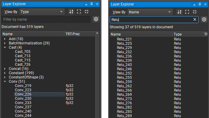
The Layer Explorer displays the list of layers currently in the model. Model layers can be organized by layer type or name, and filtered by name from the ‘Filter by name’ search box. The sort order of the layers may be toggled in the toolbar, and when organizing layers by type, all types can be expanded or collapsed from the toolbar. Layer selection is synchronized between the Layer Explorer and the canvas. Double-click on a layer in the Layer Explorer to jump to the layer in the canvas.
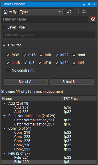
The Layer Explorer’s advanced filtering options are accessible by clicking on the gear icon next to the ‘Filter by name’ text box. The advanced filtering options allow filtering by layer type and any attributes (such as TensorRT layer precision for ONNX model) assigned to the layer. Checking a filter name enables it. The figure below shows an example of filtering for only those layers that have a precision constraint specified. A red badge with the number of active advanced filters is displayed over the Hide/Show Advanced Filters button (represented by the gear icon).
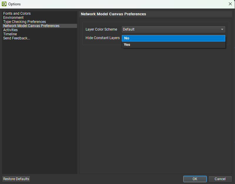
By default, constant nodes are hidden in the Model Canvas and Layer Explorer. To show constant nodes, go to View > Show All Constants. To no longer hide constants by default when opening a new model, go to Tools > Options and under the Network Model Canvas Preferences page, set Hide Constant Nodes to No.
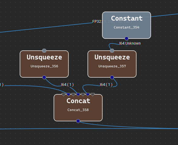
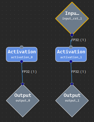
If a layer takes a constant node as an input, the input terminal connected to the constant node will be rendered in the style of a miniature constant node (a rounded gray rectangle). A single Constant node may be selectively hidden or shown by double-clicking on the terminal connected to it. The figure below shows two nodes with input terminals connected to constants: one hidden and one visible, for both ONNX and XDL models.
Parameters#
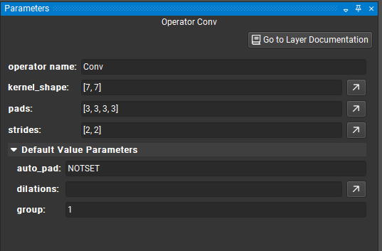
The parameter tool window allows the interactive modification of any node’s parameters. To do so, select a node from the canvas; available parameters for that operator will then be listed. The node name can also be edited but note that it must be unique across the whole graph. Parameters with unspecified values receive the operator’s default value (taken from the ONNX Opset for ONNX models, or from the XDL operator library for XDL models).
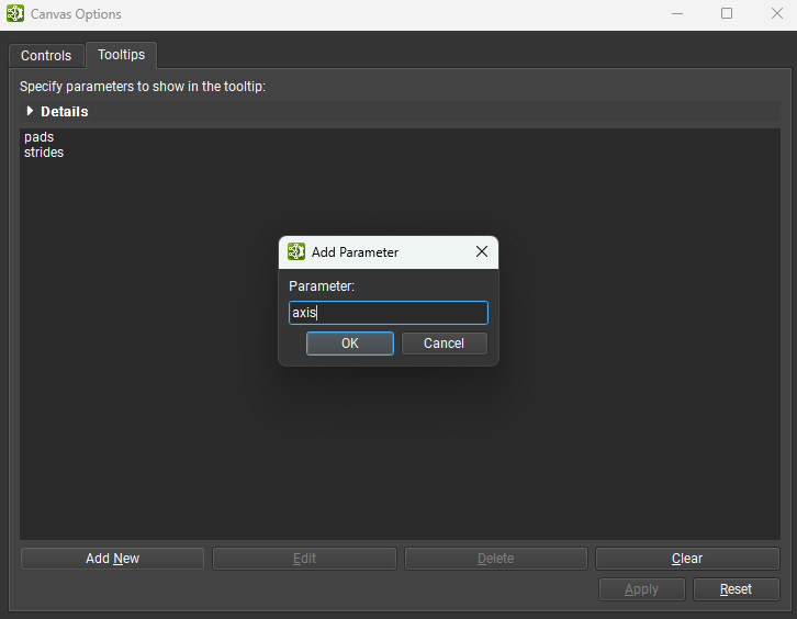
Certain parameters of interest can be added to the layer’s tooltip in the model canvas. To add a parameter by name to the node tooltip, click the model canvas options button (gear icon) in the top-right corner of the canvas and select the Tooltips tab. The image below shows a new parameter name being added to the list of parameters.
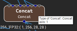
The image below shows the axis parameter for the Concat node. Note that since Concat does not have a pads or strides parameter, these are not shown in the tooltip.
ONNX Parameters#
For ONNX models, default parameters appear in the collapsible Default Value Parameters section of the Parameter Editor. When a parameter is modified, it is moved out of the default value section. To revert a parameter to its default value, click the circular arrow icon, visible on the right hand side of the parameter input field when the mouse is over the field.
Tensor/List values are expected in the following format: [1, 2, 3, 4] and can be nested for multidimensional tensors: [[1, 2], [3, 4]]. String values must be single quoted: 'Some text'. Single quotes can be embedded within string literals using \: 'It\'s alive!'.
For more advanced tensor or list editing capability, use the Tensor Editor, by clicking on the up-right arrow button at the very right of any tensor/list type parameter.
If no layer is currently selected, then model-level information is displayed, like the imported opset versions. Multiple layers can be selected at once to allow for batch parameter editing. Only parameters held in common by the selected nodes are shown.
For ONNX models, a parameter value can reference other values defined elsewhere in the model rather than holding an inline literal. The Parameter Editor exposes these references where the underlying ONNX construct allows them:
Initializer references. Operator inputs that are bound to constants are wired to a named initializer in the model. Select the input row to pick the target initializer; see the Initializer Editor chapter for managing the underlying tensors.
Attribute proto references. Inside a local function body, an attribute can be declared as a reference to one of the function’s own attributes (a
ref_attr_name) so that the call site supplies the concrete value. These references appear in the Parameter Editor when editing nodes inside a local function. See the Local Functions chapter for the surrounding workflow.
XDL Parameters#
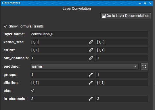
For XDL models, a parameter value can be more than a literal: it can be an expression that the XDL formula system evaluates at validation and export time. Formulas are small arithmetic and list expressions over integers, floats, strings, and references to symbolic shape variables — useful when a parameter naturally depends on another shape or on a value derived from one.
For each parameter that supports formulas, the Parameter Editor provides two input field: the first one is used to enter a formula, while the second one (read-only) shows the current evaluated value of the formula. Evaluated values can be hidden by unchecking the Show Formula Results checkbox in the Parameter Editor widget. A dedicated formula editor dialog can also be opened by clicking the pen icon next to the parameter input fields. The formula editor provides syntax highlighting and error reporting for XDL formulas, as well as a convenient list of available variables and functions.
A formula is written in the same input field as a literal value; the Parameter Editor accepts either form. For example, a kernel size can be expressed as [%{K}, %{K}] so that updating the symbolic shape K propagates to the parameter automatically.
See the XDL Formula System chapter for the full syntax — value types, operators, intrinsic functions such as POW, CEIL, FLOOR, and ABS, the %{name} variable reference form, and where formulas are surfaced in the editor (notably the Configure Dynamic Shapes dialog).
Type Check List#
Iteration on a model is a major part of the design workflow. To ensure fast and interactive iteration, the type check list reports any errors, warnings, or issues caused by the current model structure. You can double-click on any messages from the type checker to focus the corresponding operator in the canvas. This aids identification of latent issues within the model during the design process.

Nsight Deep Learning Designer provides automatic type checking of model edits:
For ONNX models, validation is performed by the Polygraphy linter.
For XDL models, validation is performed by the in-process Nsight Deep Learning Designer inner validator, which reports per-layer type errors and computes output tensor shapes.
Model validation is run automatically after any editing operation that impacted the model.
The type checker takes more time for larger models, so the validation process can be cancelled using the Cancel Check button on the top-left of the tool window. A new model validation run can be requested explicitly by clicking on the Check Model button.
Note that for very large models, automatic type checking is disabled, but explicit checking can still be performed.
Editing a Model#
Dropping an operator into the canvas creates a new instance of that operator type with an automatically generated name. All instances must have a unique name that you can edit; names should be valid C90 identifiers. Operators are represented by a rectangular node on the canvas. This node shows the name and type of the operator, as well as an icon if the type checker has reported any issues.
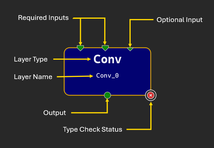
The node glyph represents the operator’s inputs and outputs using terminals. Triangles at the top of the node indicate inputs, and circles at the bottom of the node indicate outputs. Most input terminals need to be connected for the model to be valid, but optional input terminals are not mandatory. Optional inputs are represented on the glyph with a smaller triangle. Multiple links can start from a single output terminal but only one link may be connected to a given input terminal. Unconnected terminals are green and terminals with a link are dark blue. For ONNX models, input terminals connected to an initializer are rendered in light blue.
Some operators accept a variable number of input tensors to a given parameter, or produce a variable number of output tensors for a given output name. Nsight Deep Learning Designer represents these by special “infinite” terminals. Upon making a connection to an infinite terminal, more gray-colored terminals will appear between each connected terminal, representing potential new connection points. The figure below shows an example of an operator with a variable number of outputs, as well as subgraphs.
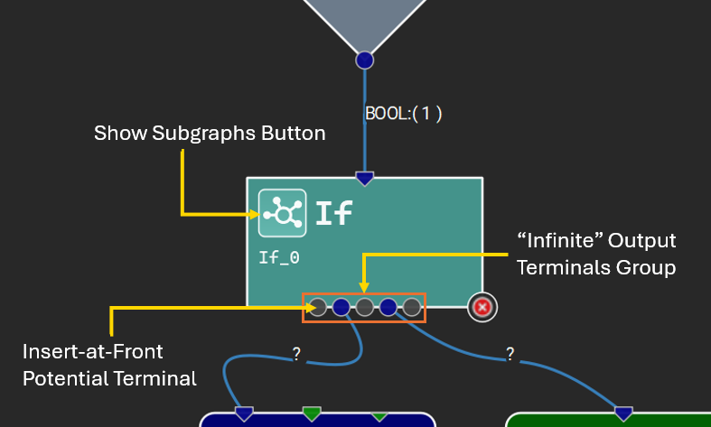
See the operator’s description in the editor’s documentation browser (Help > Layer Documentation) for details of a specific operator’s inputs and parameters.
To connect node A to node B, click and drag from any input terminal on node A to any output terminal on node B (or from any output terminal on node A to any input terminal on node B). This action creates a link. Operators and links can be removed by selecting them and using the delete key. Upon successful model validation, intermediate tensor sizes are calculated and displayed alongside the corresponding link.
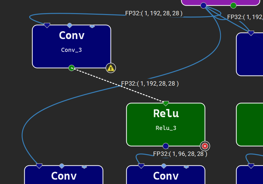
Nodes are automatically laid out when a model is loaded, and can be rearranged freely by clicking and dragging the nodes on the canvas. The background grid can be turned on with View > Show Grid to help align layers.
Double-clicking an unassigned input or output terminal on a node will create an input or output operator automatically and link it to that terminal.
XDL Specific Model Design#
The following sections describe features specific to XDL models in Nsight Deep Learning Designer.
Model Variables#
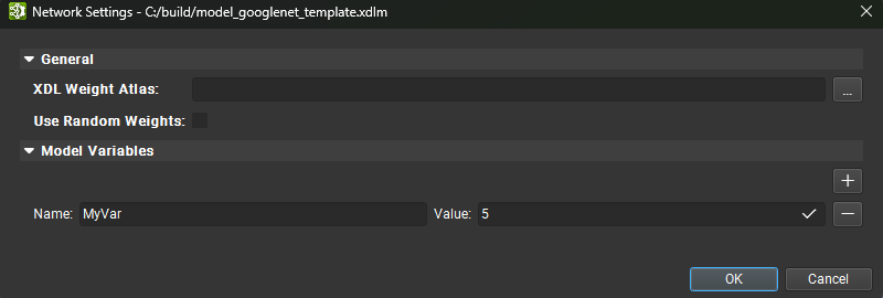
XDL models support declaring and using model variables — named symbolic values that can be used in formulas across the model. Model variables are defined in the Network Settings dialog, available from the Tools menu, or from the Parameter Editor when nothing is selected on the canvas.
To define a model variable, open the Network Settings dialog and navigate to the Model Variables section. Click the + button to add a new variable, then enter its name and value. The value can be any formula that resolves to a valid type. Variables can also reference other variables, as long as there are no circular dependencies.
Once defined, a model variable can be used in any formula by referencing its name with a %{} syntax — for example, %{MyVar1}.
Dynamic Shape Support#
XDL models support dynamic shapes — dimensions that are not fixed to a literal integer but can vary at runtime. Dynamic shapes are represented by symbolic shape variables. This allows for more flexible models that can be parameterized for different input sizes.
Symbolic shapes come in three flavors, distinguished by how their value is produced:
- DataDependentSize
The shape value depends on a dynamic value carried inside a tensor at runtime — for example, a stop scalar passed to an
Arangeoperator. The runtime value is not available at edit time, so XDL requires a user-supplied formula hint that stands in for it during validation and export.- DynamicSize
The shape is an arithmetic expression over at least one other symbolic shape — for example,
%{N} * 2or%{H} + %{Pad}.- ConditionalSize
The shape cannot be expressed as a single arithmetic expression — typically the result of a conditional branch. The value still depends on at least one other symbolic shape, it is recorded as a constraint rather than an evaluable formula.
The Configure Dynamic Shapes dialog available from the Tools menu provides a convenient interface inspect symbolic shapes in the model and provide hints for DataDependent shapes.
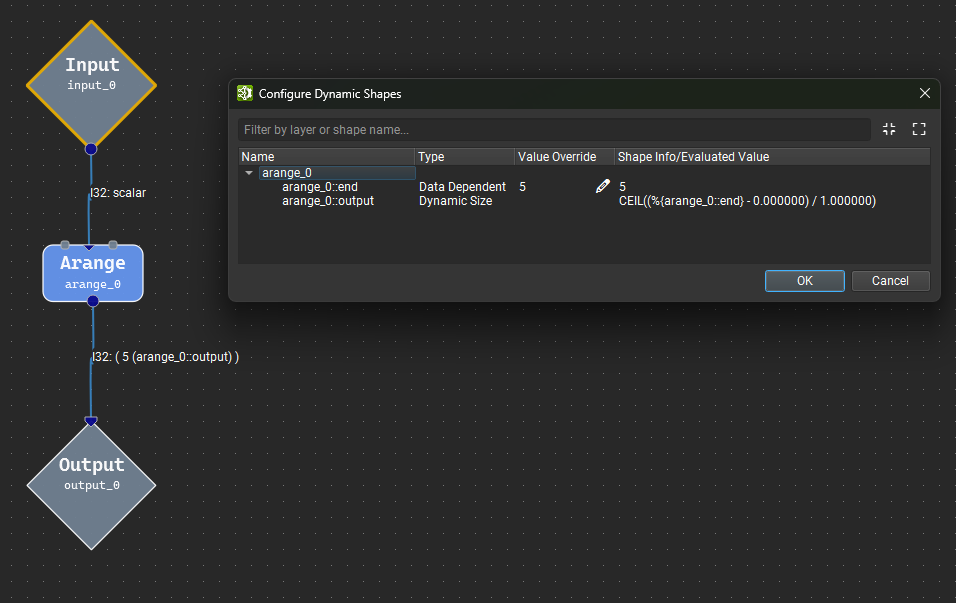
The dialog lists all symbolic shapes in the model, their flavor, and the current formula hint if applicable. Only DataDependent shapes can have a formula hint.
In the canvas, any output shape that is symbolic will display the symbolic name and the current evaluated value if available based on the user-provided hints.
ONNX Export#
When exporting to ONNX, symbolic shapes must be resolved to concrete values through the user-provided formula hints. If a symbolic shape cannot be resolved to a concrete value, the export will fail with an error message indicating the offending shape and the formula hint that could not be resolved.
Templates#
A template is a named, reusable group of XDL operators. Templates capture the repeated module structure that is typical of deep-learning models — a residual block, an attention head, a downsampling stage — so the same pattern appears once in the document rather than once per instantiation.
Templates serve a similar role as a PyTorch nn.Module subclass in source code or a local function in ONNX. Templates are stored inline in the .xdlm file.
Creating a New Template#
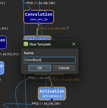
To create a template, select a group of operators in the canvas and click Group in the right-click context menu. After providing a unique name, the selected operators will be replaced by an instance of the new template.
Instancing a Template#
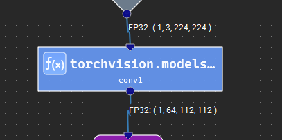
Templates are defined at the model level and can be instantiated like any other operator from the Layer Palette. Template instances can be recognized in the canvas by their blue background color, square edges, and f(x) symbol. Clicking on the symbol will open the template definition in a separate document inside of Nsight Deep Learning Designer.
If a template has parameters, these will be listed in the Parameter Editor when selecting an instance of that template in the canvas, see the next section for details.
Editing a Template#
Once opened in Nsight Deep Learning Designer, a template can be edited just like a normal model. Changes made to a template must be applied by using the Confirm Template Edits button on the main toolbar. Once applied, the template definition will be updated in the model.
Additionally, templates can be parameterized. When editing a template in Nsight Deep Learning Designer the Template Definition Settings dialog can be opened using the Tools > Template Settings action or using the Edit Template Scoped Variables button from the Parameter Editor when no nodes are selected.
From this dialog, new parameter can be defined using the + button. A unique name and a default value (as a formula) must be provided. Parameters can also be removed by clicking on the respective - button.
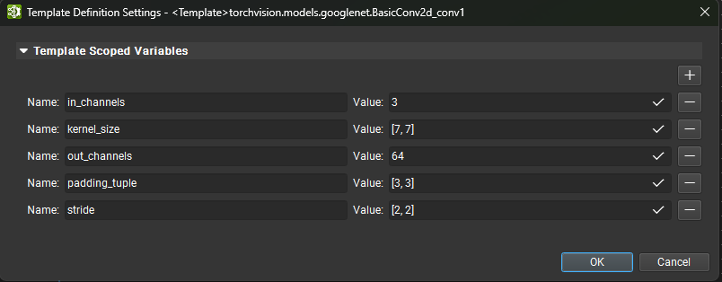
Operators that are part of a template may use template parameters as formula variables in their parameter values using the %{name} syntax. When a template parameter is updated, all operators that reference that parameter will be updated as well.
Inspecting Template Instances#
When inspecting a template definition in Nsight Deep Learning Designer, it is possible to set the context to a specific instance of that template. This will update all template parameter values to reflect the values provided by that instance as well as set input sizes, allowing the type checker and output shape inference to report values as they would be for that instance. To set the context to a specific instance, click on the Configure Template Context action from the Tools menu.
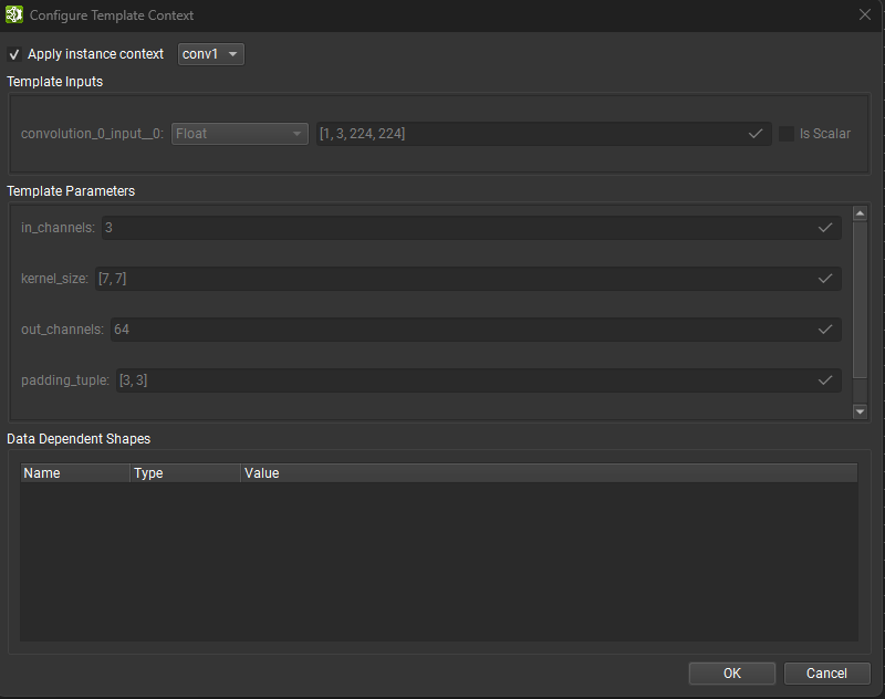
From this dialog, you can select the template instance to use as context from the drop-down list, or manually override parameter values, input shapes, and data dependent shapes. Clicking Ok will apply the context and update the graph validation results accordingly.
Source Information#
When an XDL model is produced from a PyTorch source using the nsight-pytorch2xdl importer, each operator can carry source provenance — the originating Python file, line number, and function name. This metadata travels with the model as long as it is saved in XDL form, so you can trace any layer on the canvas back to the source code that produced it.
What Source Information Records#
Source information is attached at import time by nsight-pytorch2xdl. For each operator the importer emits, it records:
File — the Python source file containing the call that produced the operator.
Line — the line number within that file.
Function — the name of the enclosing function or method (typically the
forwardmethod of annn.Module).
For a model produced by torch.compile on a ResNet subclass, for example, a single convolution layer might be tagged with the line in forward() where the corresponding self.conv1(x) call is made.
Source information is optional. XDL models produced by other means (manual edits, programmatic graph construction without source annotation) simply omit the metadata; the canvas behaves normally but the source-jump action is not offered for those layers.
What the Editor Displays#
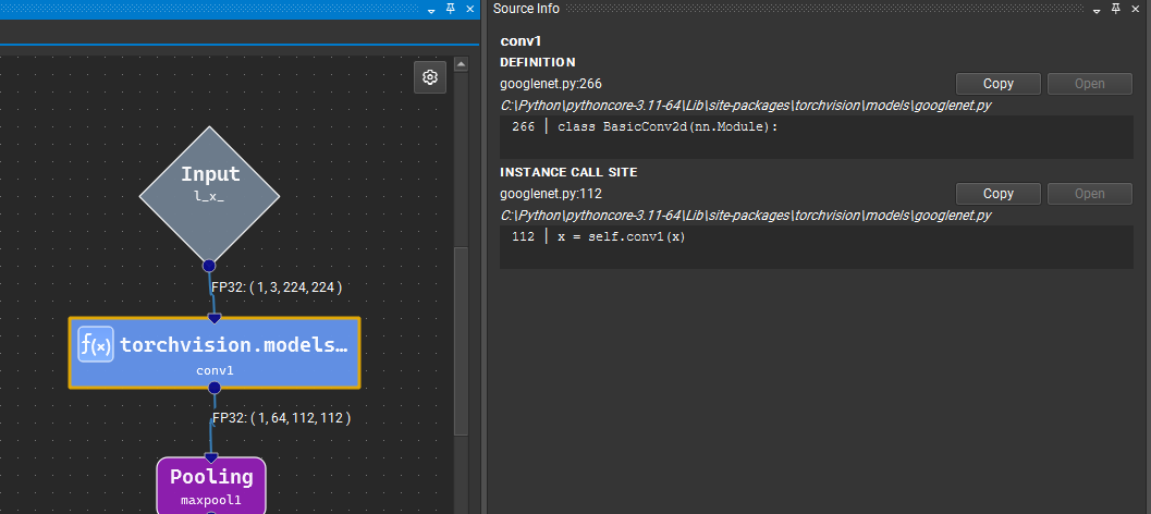
Nsight Deep Learning Designer surfaces source information in the Source Info tool window, available from the View > Tool Windows menu. When an operator with source information is selected in the canvas, the tool window displays the file path, line number, and function name for that operator. If the file is accessible on the local filesystem, an Open button will be enabled, to open the file in the system’s default editor for Python files.
For template instances, the source information shows both the definition site and the instantiation site.
Source information is preserved when you save the model. Editing a layer’s parameters does not invalidate its source location.
ONNX Specific Model Design#
The following sections describe features specific to ONNX models in Nsight Deep Learning Designer.
Initializers#
Initializers are used in ONNX to represent constant tensor values such as weights. They can be used directly as inputs without introducing an extra Constant operator. A single initializer can be used by multiple operators in the graph. Initializer values can either be embedded directly in the ONNX model or referenced from an external binary file. Each initializer is identified by a unique name within the model.
In Nsight Deep Learning Designer, the Initializer Editor tool window allows the user to view and edit the initializers of an opened ONNX model.
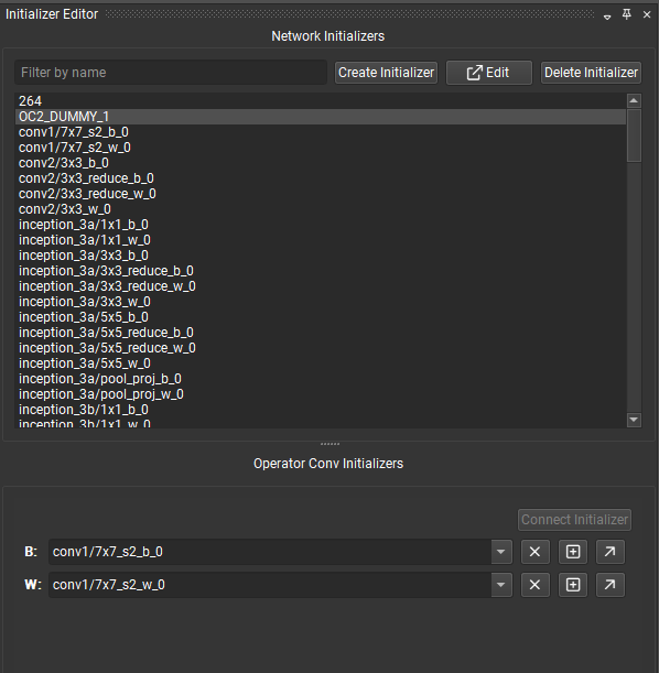
The initializer editor is divided in two parts: an upper section for viewing, creating, editing, and deleting any of the initializers in the model, and a lower section for viewing and connecting the initializers of the currently selected node. If no node is currently selected, the lower section will be hidden.
The network initializer list can be filtered by name. The selected initializer can be:
Removed from the model which will also disconnect them from any node currently using it.
Edited using the Tensor Editor.
Double-clicking an initializer in the list will select and center in the Model Canvas the nodes currently connected to the initializer.
An initializer can be created from scratch with the dialog opened using the Create Initializer button.
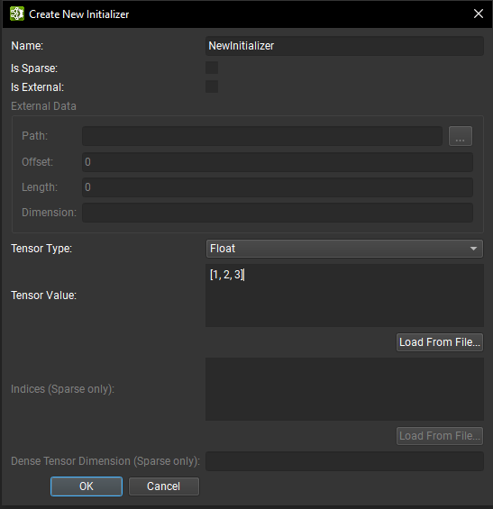
From there, the initializer information can be provided such as the name, tensor type, and tensor value. Tensor values are expected in the following format: [1, 2, 3, 4] and can be nested for multidimensional tensors: [[1, 2], [3, 4]]. String values must be single quoted: 'Some text'. Single quotes can be embedded within string literals using \: 'It\'s alive!'.
Tensor values can be loaded from a NumPy file. Note that the data type must match the one from the NumPy file before loading.
Initializers can also be generated for placeholder purposes using either random or zeroed data. Choose a tensor type from the Create New Initializer dialog and press the Generate… button. Not all tensor types currently support random generation; the button is disabled if no generation support is available.
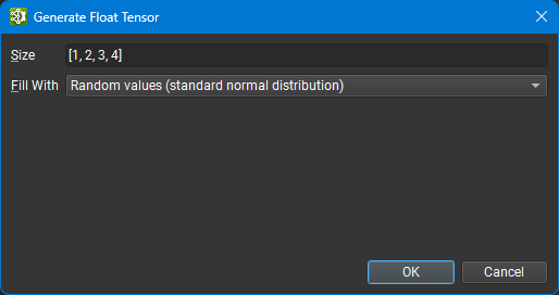
Enter a size for the tensor in [1, 2, 3, 4] format and choose the fill method:
Random values (standard normal distribution) uses a standard normal distribution (mean = 0, variance = 1). Available for floating-point types that use more than one byte for storage.
Random values (uniform distribution) uses a uniform distribution across the range supported by the type. Available for all four-bit, integer, and Boolean types.
Zero values sets each element of the generated tensor to zero. Available for all types.
Random positive values (uniform distribution) uses a uniform distribution across all positive values supported by the type. Excludes zero. Available for all integer types that use at least one byte for storage.
Random negative values (uniform distribution) uses a uniform distribution across all negative values supported by the type. Excludes zero. Available for signed integer types that use at least one byte for storage.
Random positive values (normal distribution) uses the absolute value of a standard normal distribution to generate positive values, clamping to
FLT_MINto exclude zeros. Available for floating-point types that use more than one byte for storage.Random negative values (normal distribution) uses the absolute value of a standard normal distribution to generate negative values, clamping to
-FLT_MINto exclude zeros. Available for floating-point types that use more than one byte for storage.
If the initializer is sparse, then in addition to the non-default value tensor, an indices tensor and dense tensor dimension must be provided. See ONNX SparseTensorProto specification for more information on the format expected by ONNX.
If the initializer is marked as external, a path to a binary file on disk must be provided. The external file must be at a location relative to where the model is stored. For that reason, it is not possible to create an external initializer when working on an in-memory only model, such as an unsaved new model. Offset is the byte location within the file at which the stored data begins, and length is the number of bytes containing data. External initializer tensor data are not stored directly in the ONNX model. This can reduce the size of the model file.
When selecting a node from the canvas and if it has a free terminal, the Connect Initializer button is enabled to allow connecting a model initializer to it. Once connected, the terminal will change to a yellow color on the node glyph, indicating that it is connected to an initializer. Connecting a link to it will disconnect the initializer from the node input.
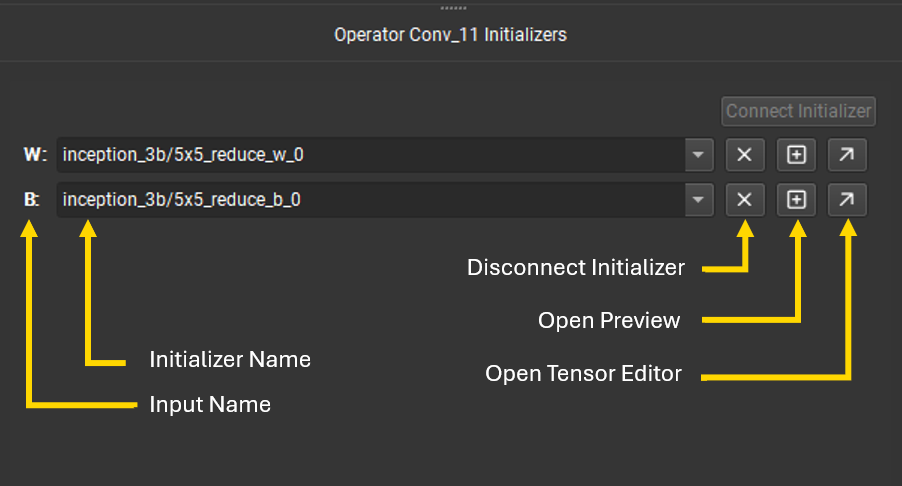
The bottom part of the initializer editor lists all terminals of the currently selected node which are connected to initializers. The initializer used by a terminal can be switched using the drop-down menu. The drop-down is filterable by name. Using the cross button, the initializer can be disconnected from the terminal. The plus button opens a preview of the tensor values and the diagonal arrow button will open the Tensor Editor.
Tensor Editor#
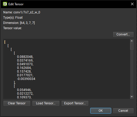
ONNX tensor data may be modified with the Tensor Editor. Tensor values can be directly edited and the tensor dimension will be updated automatically once the edit is validated. If the tensor has more than ten thousand elements, it is not editable but the tensor value can still be updated with a NumPy file. The current tensor data can also be exported to a NumPy file for external processing.
In the case of a sparse tensor, the indices and dense tensor dimension can be modified. For external tensors, the path, offset, and length information can be edited. In all cases, only the name of the initializer cannot be modified.
It is possible to convert a tensor’s data to a different data type by using the Convert button; the only exceptions are external data and tensors of Boolean or string type. The data type conversion dialog lists all available data types to which the tensor can be converted. Note that depending on the source and target conversion data type, data precision loss and/or truncation can occur.
Subgraphs#
Some ONNX control flow operators such as Loop and If take one or more subgraphs as parameters. Subgraphs are ONNX graphs that share initializers and imported opsets with their containing model.
The scope of a subgraph is determined by its parent, whether that be an operator instance or local function definition. All subgraphs within a scope must have unique names.
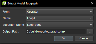
Subgraphs can be exported to a standalone ONNX model in Nsight Deep Learning Designer by using the Tools > Extract Model Subgraph command. Within the dialog that opens, select the subgraph by identifying the type of its parent (operator or local function), the name of its parent scope, and the subgraph name within that scope. Then choose an output path for saving the extracted subgraph.
Only operators from the current document are listed. To export subgraphs from operators inside another subgraph or local function, the Tools > Extract Model Subgraph wizard must be opened from the corresponding subgraph or local function document.
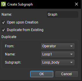
A subgraph can be created from scratch using the + button next to an operator parameter of subgraph type. In the creation dialog, a unique subgraph name given its scope must be provided. Some options can be enabled both to open the subgraph once created, as well as to duplicate an existing subgraph from an operator or local function subgraph.
For parameters of subgraph list type, a list view shows all the graphs contained in the parameter list, and the + button can be used to create and add a new subgraph to the list, while the - button will remove the selected subgraph. Using the up-right arrow button, the currently selected graph can be opened in a separate document inside Nsight Deep Learning Designer.

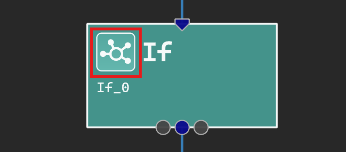
Subgraphs can be visualized in separate document tabs. To open a subgraph, click on the subgraph button on the operator glyph and select the desired subgraph from the menu, or click on the subgraph’s link within the Parameter Editor tool window. The subgraph button is shown boxed in red below.
Once opened, subgraphs can be edited within Nsight Deep Learning Designer just like a normal ONNX model, though model initializers do not have an analog within subgraphs and therefore cannot be edited. Preserve changes within a subgraph within the enclosing document using the Confirm Subgraph Edits button on the main toolbar. This command updates the parent document to reflect changes to the subgraph. Parent documents are otherwise read-only while their subgraphs are open for editing.
Local Functions#
Graph components are commonly repeated within a model. Local functions can be used to represent these recurring patterns. This creates a higher-level representation of the model by abstracting the patterns as single nodes.
Local functions are defined at the model level and can be instantiated like any other operator type from the Layer Palette. Local function instances can be recognized in the canvas by their black background color, square edges, and f(x) symbol. Clicking on the symbol will open the function definition in a separate document inside of Nsight Deep Learning Designer.
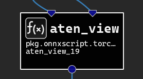
Once opened in Nsight Deep Learning Designer, a local function can be edited just like a normal model, apart from creating or removing model initializers. Changes made to a local function must be applied by using the Confirm Local Function Edits button on the main toolbar. Once applied, the local function definition will be updated in the model.
Additionally, local functions can be parameterized. When editing a function in Nsight Deep Learning Designer the Local Function Definition Settings dialog can be opened using the Tools > Local Function Settings action or using the Edit Local Function Parameters button from the Parameter Editor when no nodes are selected.
From this dialog, new parameter can be defined using the + button. A unique name must be provided as well as the parameter type. A parameter of type undefined requires that each instance of the function provides a type of information when passing a value for this parameter. Otherwise, a default value must be provided for all other types. Parameters can also be removed by clicking on the respective - button.
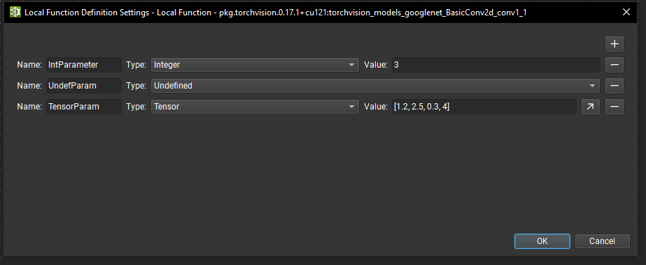
Operators that are part of a local function may reference parameters provided to the enclosing function instead of providing a specific parameter value. Operators with parameter references will use the corresponding reference value provided by the local function instance.
When selecting an operator, its parameters can be assigned to a reference using the Set Reference Parameter button at the top of the Parameter Editor. A dialog opens with a drop-down list containing available parameters of this operator which do not already use references. The second drop-down list contains all the available local function parameters that can be used as a reference.
Local function parameters of an incompatible type are grayed out and cannot be selected. Reference assignments are validated when the dialog is closed.
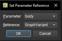
Reference parameters are represented with a drop-down list in the Parameter Editor. The current reference can be directly switched using the drop-down control. The reference can be removed using the X button; this reverts the parameter back to its original type and default value.
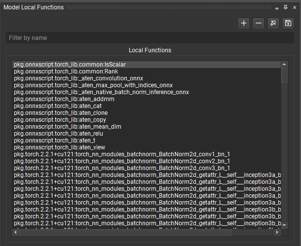
Local functions can be managed using the Model Local Functions tool window. It lists all functions currently defined in the model, the list can be filtered by name.
The selected function can be opened or extracted to a standalone ONNX model using the arrow and save buttons respectively.
The + button allows you to create a local function from scratch. You must first provide a function name and domain. Finally, local functions can be deleted from the model using the - button. All instances of that function will be transformed into custom operators.
Operations on ONNX Models#
Batch Modifications#
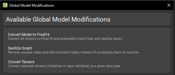
In certain workflows it can be necessary to modify large portions of an ONNX model or perform specific modifications upon every node. Nsight Deep Learning Designer has batch modification actions for some common use cases. They can be found under the Tools > Global Model Modification dialog.
Convert Model to FP16#
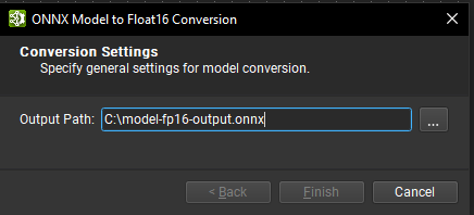
A common model optimization technique is to convert model weights to a half-precision format (such as FP16). This can decrease the model size by as much as half and improve performance on some GPUs, at the potential cost of some accuracy.
Using Nsight Deep Learning Designer’s Convert Model to Float16 batch modification action under the Tools > Global Model Modification dialog, an ONNX model can be converted to use Float16. Provide an output path for the converted model and click Finish. A spinning wheel will appear while conversion is being performed. When the process is finished, a dialog box will show the status of the conversion with an expandable section containing detailed logs.
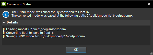
Nsight Deep Learning Designer’s Float16 conversion is provided by Polygraphy convert subtool, which converts initializers and tensors to Float16 when applicable and can insert Cast operators to maximize the number of operators that will be running with Float16 data.
Sanitize Graph#
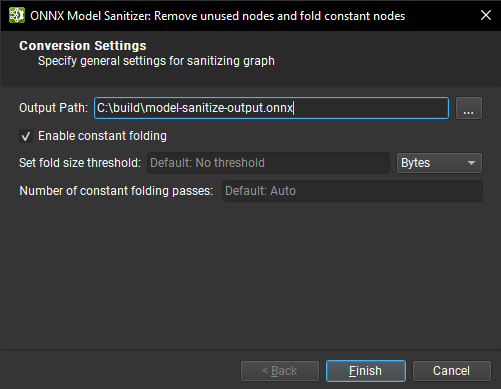
The Sanitize Graph batch modification action, under the Tools > Global Model Modification dialog, can help reduce an ONNX model’s size by performing constant folding and removing unused nodes.
To perform graph sanitization, provide an output path for the sanitized model in the dialog and click Finish. A spinning wheel will appear while sanitation is being performed. When the process is finished, a dialog box will show the status with an expandable section containing detailed logs.
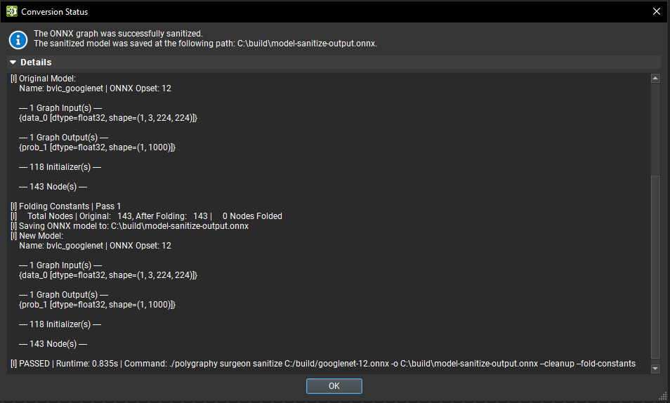
The conversion is provided by the Polygraphy sanitize subtool.
Some options are available:
Enable Constant Folding: On by default. If off, no constant folding will be performed.
Fold size threshold: Sets the maximum per-tensor size threshold, in bytes, for which to apply constant folding. Any nodes generating tensors larger than this size will not be folded away.
Number of passes: Sets the number of constant folding passes to run. Subgraphs that compute tensor shapes may not be foldable in a single pass. If left empty, Polygraphy will determine the number of passes necessary.
Convert Tensors#
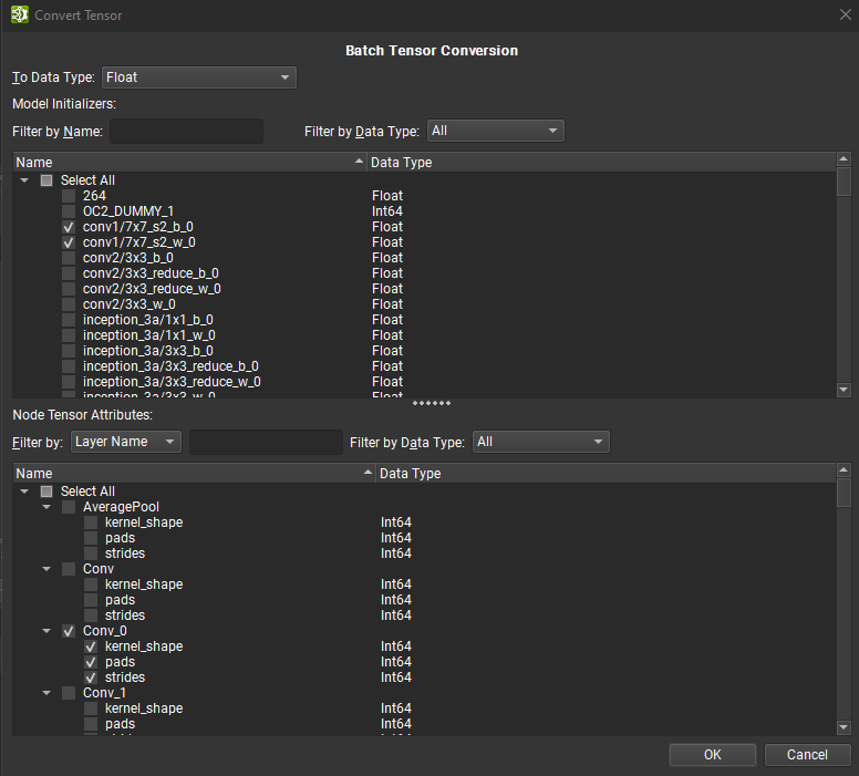
Multiple tensors may be converted as a batch by using the Batch Tensor Conversion dialog. To access this dialog, open the Tools > Global Model Modifications dialog, and then click Convert Tensors. Individual tensors can be converted inside the Tensor Editor.
The batch tensor conversion dialog is separated in two panels: the top one lists all model initializers while the bottom part contains all tensor or list based node attributes. Initializers can be filtered by name and data type, while node’s tensor or list can be filtered by node or tensor name and data type.
A mix of node tensors, lists, and initializers can be selected for conversion to a single target data type, using the combo box at the top of the dialog. Once all the necessary tensors have been selected, click OK to start batch conversion. A dialog will show the progress of the conversion and any errors observed during the process.
Depending on the source and target conversion data type, data precision loss and/or truncation can occur. Note that undoing the batch conversion will revert all previously converted tensors to their original data type and values.
Inserting Quantize/Dequantize Nodes#
For ONNX models using Opset 13 or higher, Nsight Deep Learning Designer can automatically insert paired QuantizeLinear and DequantizeLinear nodes around a selected subset of the nodes in a graph. The effect of these paired quantizations and dequantizations is to simulate the effect of quantizing to the target type. TensorRT may use this information to create fused quantized kernels to improve performance. To use the Add Q/DQ Nodes operation, select a set of nodes in the model canvas, right click, and select Add Q/DQ Nodes from the context menu.
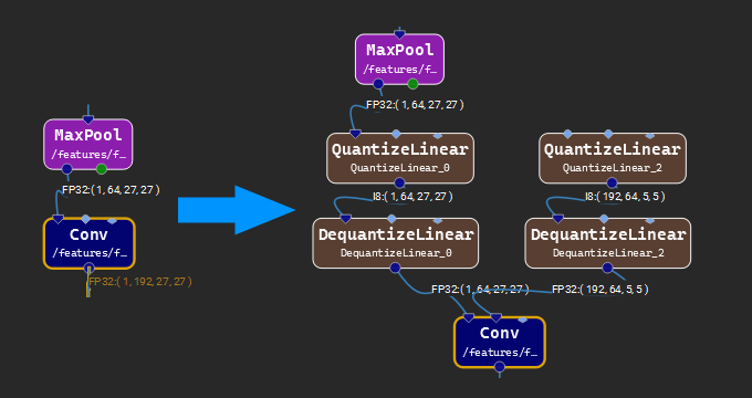
The image above shows the inserted quantize/dequantize nodes inserted at the edge of the selection and into initializer connections. Typically, one should select a small handful of nodes which could be fused into a single quantized kernel.
Parameters#
The Q/DQ dialog, shown below, lets the user specify how the operation is to be performed. The operation acts on two types of tensors: initializers connected to nodes in the selected subset of the graph, and activations that cross the selected/unselected nodes boundary. Whole-tensor quantization is applied to all activations of an eligible type, using the user-supplied Scale Factor and zero for the zero-point. Activations of an unsupported type are not quantized. Certain initializers are quantized along a particular axis: Conv W is quantized along axis 0 (the number of feature maps), MatMul A and B along axis 0 and axis 1, respectively. Initializers with no specific axis quantization rule are subject to whole-tensor quantization.
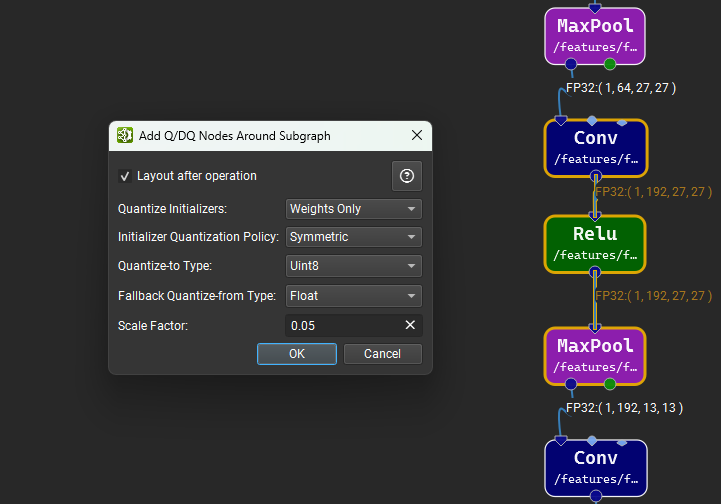
The sections below provide more details on each parameter seen in the dialog.
Quantize Initializers#
This parameter controls which initializer connections used in the selection region will have Quantize/Dequantize pairs inserted. When an initializer is “quantized”, it will be disconnected from its input on the node, and connected to a newly inserted QuantizeLinear node, which will in turn be connected to a DequantizeLinear node, the output of which will connect to the original initializer input index on the node. Regardless of the option chosen, initializers of an unsupported type will be left unchanged.
- None
No initializers will be quantized.
- Weights only (Default)
Only known weight initializers (e.g. Conv W, MatMul A and B, etc.) will be quantized.
- All but biases
All initializers except for known biases (e.g. Conv B input) will be quantized.
Initializer Quantization Policy#
When an initializer is to be quantized, this parameter controls the scale factor inputs for quantization. The zero vector is used for all zero-point inputs, regardless of policy.
- User Scale Factor
The scale factor is the value supplied in the Scale Factor field of the dialog. If the initializer is to be quantized along an axis, the user scale factor will be broadcast to a vector of the appropriate size.
- Symmetric (Default)
The scale factor is computed automatically from the maximum absolute value along the quantization axis. If there is no quantization axis, the maximum absolute value of the initializer is used.
Quantize-to Type#
This specifies the type to which quantization is being simulated by the Q/DQ pairs. The following types are supported (Opset permitting):
Uint8 (Note: Not supported by TensorRT)
Int8
Float8E4M3FN
Float8E4M3FNUZ
Float8E5M2
Float8E5M2FNUZ
Fallback Quantize-from Type#
The fallback type to use when the type of an activation tensor cannot be inferred. Nsight Deep Learning Designer infers the type of activation tensors (links) as part of the type checking and inference process. This process may fail due to errors in the model, or may not have been run if the model is very large. If the process fails, Nsight Deep Learning Designer will assume that any activation tensors are of the type specified here.
Scale Factor#
A user-provided positive floating-point number that will be used as the scale factor for the quantization of activations, and if the initializer quantization policy is set to User Scale Factor, the initializer scale factor will be set to this value.
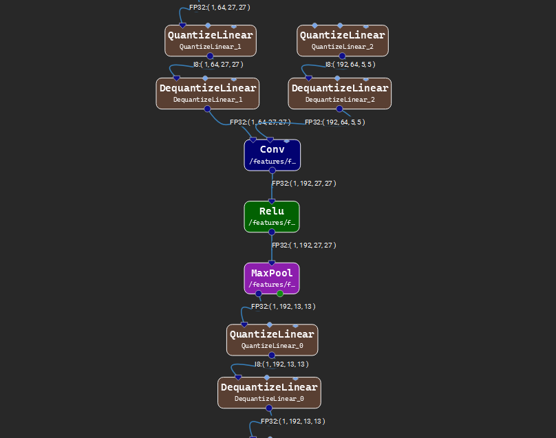
The image above shows the result of running the Add QDQ Nodes operation on the selected nodes. The operation can be undone from the Edit menu.
The XDL Format#
XDL (“eXtensible Deep Learning”) is Nsight Deep Learning Designer’s native model format. It is an XML-based ONNX alternative that provides streamlined interactive editing in the model canvas, interoperability with PyTorch, and high-level abstractions like reusable templates (analogous to PyTorch nn.Module) and formula-based parameters.
XDL models can be opened, edited, and saved directly in Nsight Deep Learning Designer. They are exported to ONNX (via the built-in validator) when an inference engine such as TensorRT or ONNX Runtime is needed.
File Extensions#
An XDL model is split across two files:
.xdlm— the XDL model. An XML document describing the operator graph, parameters, templates, and optional source-info metadata..xdlw— the XDL weights archive. A ZIP file containing the binary tensors for each weight in NumPy format, plus per-tensor metadata. The weights file is optional: a graph that uses only random or input-provided weights does not need one.
The two files are conventionally named with the same base (for example Resnet32_Model.xdlm and Resnet32_Model.xdlw) and kept side by side.
When to Choose XDL vs. ONNX#
Both formats are fully supported by Nsight Deep Learning Designer. Use this table as a starting point:
Aspect |
XDL |
ONNX |
|---|---|---|
Wire format |
XML |
Protocol Buffers |
Reusable modules |
Templates (first-class) |
Local Functions |
Source-line provenance |
Built in ( |
Not represented |
Inference |
Exported to ONNX for TensorRT / ONNX Runtime |
Consumed directly |
Typical use case |
Iterative authoring, PyTorch round-trip |
Deployment and profiling |
Choose XDL when you are working with PyTorch, want to preserve module structure across save and load, or rely on jumping from the canvas back to source. Choose ONNX when you are consuming a model produced elsewhere or want to edit the same artifact that will be deployed.
XDL Formula System#
The XDL formula system lets parameter values and dynamic-shape values be expressed as small arithmetic and list expressions instead of fixed literals. Formulas are resolved by Nsight Deep Learning Designer at validation and export time, so the surrounding model stays consistent when a single symbolic shape changes.
Use a formula whenever a parameter naturally depends on other shapes or values.
Value Types#
A formula evaluates to one of the following types:
nil— absent value.boolean —
trueorfalse.integer.
float.
string.
dimension — a value that participates in shape arithmetic.
numeric list — a homogeneous list of integers or floats.
string list — a homogeneous list of strings.
generic list — a mixed-type list, used when entries differ.
Literals#
Integers. Written without a decimal point or exponent:
1,-3,156.Floats. Written with a decimal point or an exponent:
2.5,1e2,1e-2.Booleans.
trueorfalse.Strings. Single-quoted:
'ReLU'. An embedded single quote is escaped with a backslash:'It\'s alive!'.Lists. Comma-separated and bracketed:
[1, 2, 3]. Lists nest:[[1, 2], [3, 4]].
Operators#
Arithmetic uses the standard infix operators +, -, *, /, the unary minus -, and parentheses ( and ) for grouping. Mixed integer-and-float arithmetic promotes to float, as in most expression languages.
Intrinsic Functions#
The formula system provides a small set of built-in functions:
ABS(x)— absolute value ofx.POW(base, exponent)—baseraised toexponent.CEIL(x)— ceiling ofx.FLOOR(x)— floor ofx.
Variables#
A variable is referenced as %{name}. The resolver maintains the current set of variables and their values;
Variables may also be substituted inside a single-quoted string literal. The expression 'output_%{layerIdx}_dim' evaluates to the string output_0_dim when layerIdx is 0, and tracks layerIdx as it changes.
Examples#
The following formulas illustrate common expressions:
1 + 3                       => 4                  (integer)
5 / 2                       => 2.5                (float)
POW(2, 3)                   => 8                  (integer)
CEIL(2.1)                   => 3                  (integer)
%{MyVar1} * 2               => integer            (depends on MyVar1)
[%{MyVar1}, %{MyVar3}]      => dimension list
'output_%{layerIdx}_dim'    => substituted string
Grammar Reference#
The following is the formal grammar for XDL formulas, in EBNF form:
boolean  = 'TRUE' | 'FALSE' ;
numeric  = double_ ;
text     = ( unicode_char_ | escaped_seq )+ ;
escaped_seq = ( '\\' , ('x' | 'u' | 'U') , hex_ );
quotedText = '\'' , ( text | variable )+ , '\'' ;
identifier = [A-Za-z_] , ([A-Za-z0-9_])* ;
variable = '%{' , identifier , '}';

expression = term , (('+' , term) | ('-' , term))* ;
term       = factor , (('*' , factor) | ('/' , factor))* ;
factor     = numeric | variable | funcCall
        | '(' , expression , ')'
        | ('-' , factor)
        | ('+' , factor) ;

funcCall  = identifier , '(' value , (',' , value)* , ')' ;

list            = '[' , listExpr , (',' , listExpr)* , ']' ;
listExpr        = listFlattenExpr | value ;
listFlattenExpr = 'FLATTEN(' , value , (',' , value)* , ')' ;

value = boolean | list | expression | quotedText ;
XDL Weights Archives#
XDL stores weights separately from the graph. A trained XDL model is conventionally distributed as a .xdlm file (the graph) paired with a .xdlw file (the weights). Keeping the two files separate lets you swap weight sets without changing the graph, and keeps the textual XML model file small and diff-friendly.
A .xdlw file is a standard ZIP archive. Inside, it contains:
One binary tensor per weight. Each tensor is stored as a NumPy array, named after the corresponding weight layer in the
.xdlm.
A .xdlw is produced by the PyTorch importer (nsight-pytorch2xdl) when weights and export_weights are supplied to export_to_xdl. The importer extracts the values from the provided weights, often the model state_dict, and emits a matching archive. See the PyTorch Exporter and Importer chapter.
Using Weights at Export Time#
When you export an XDL model to ONNX, set the weights path to the xdlw file under the Network Settings dialog. This will cause the weights to be included in the ONNX export, so they are available to the inference engine.
PyTorch Exporter and Importer#
Nsight Deep Learning Designer includes utilities for converting model representations between XDL and PyTorch.
The importer converts a PyTorch nn.Module into an XDL model file that can be opened in Nsight Deep Learning Designer. The exporter generates PyTorch source code from an XDL model.
PyTorch Import#
To open a PyTorch model in Nsight Deep Learning Designer, convert the PyTorch nn.Module into an XDL model first. The importer is provided as a Python package available through PyPI: pip install nsight_pytorch2xdl.
How the Import Works#
The importer does not parse Python source directly. Instead, it:
Runs
torch.compile(..., fullgraph=True)internally to ask TorchDynamo for a single compiled graph.Captures the resulting Torch FX graph.
Walks that FX graph and maps supported operations into XDL operators.
Can build two forms of the converted network: one flattened graph with module structure expanded into ordinary operators, and one template-oriented graph that reconstructs reusable module structure where possible.
Because the importer uses fullgraph=True, graph breaks are not allowed. If TorchDynamo cannot capture the model as one FX graph, conversion fails instead of silently splitting the model into multiple compiled regions.
Common causes of graph-break-related failures include unsupported Python control flow, unsupported data-dependent operations, unsupported logging or side effects inside the compiled region, and other operations that TorchDynamo cannot trace as part of a single graph. For background, see the PyTorch documentation on Working with Graph Breaks and Use fullgraph=True to Identify and Eliminate Graph Breaks.
The importer does filter out certain compile-time-only checks such as torch._check-style assertions so those nodes do not appear in the generated XDL graph.
The PyTorch importer can emit an XDL model in either of two forms:
- Template-oriented
Repeated module structure is preserved. Each module instance becomes a reference to a single template definition. The canvas shows the module as a composite node; you can open the template definition to see and edit its body. Provide an output path for this form using the
template_save_pathargument to the importer API. This is the recommended form for editing.- Flattened
Every template instance is expanded into plain operators. The model becomes a single flat graph with no template references. Flattened graphs are easier to consume from tools that do not understand templates, and are the form passed to the validator when exporting to ONNX. Provide an output path for this form using the
flatten_save_pathargument to the importer API.
A typical workflow is:
import torch
import torch.nn as nn
from nsight_pytorch2xdl import PyTorch2XDL

# Define a simple PyTorch model
class SimpleModel(nn.Module):
    def __init__(self):
        super(SimpleModel, self).__init__()
        self.linear = nn.Linear(10, 5)

    def forward(self, x):
        return self.linear(x)

# Instantiate the model and set it to evaluation mode
model = SimpleModel()
model.eval()

# Prepare an example input tensor shape (1, 10)
example_input_shapes = [[1, 10]]

# Export the model to XDL format, the exported files will be saved to the specified paths
PyTorch2XDL.export_to_xdl(model, network_name="SimpleModel", input_shapes=example_input_shapes, flatten_save_path="path/to/folder", template_save_path="path/to/folder")
Importer API#
The main entry point is:
PyTorch2XDL.export_to_xdl(
 model: torch.nn.Module,
     *,
 network_name: str | None = None,
 input_shapes: List[List[int]] = [],
 input_data: Iterable[Any] | None = None,
 input_tensor_device: str = "cpu",
 weights: Any = None,
 schema: str | None = None,
 export_weights: bool = True,
 flatten_save_path: str | None = None,
 template_save_path: str | None = None,
 log_level: int = verboselogs.NOTICE,
 merge_stacks: bool = True,
 include_source_metadata: bool = True,
 **kwargs: Any,
 )
Importer Options#
The importer supports the following arguments:
modelThe PyTorch module to convert.
network_nameOptional name for the generated XDL network. If not provided, the importer uses the PyTorch class name of the root module.
input_shapesThe input tensor shapes used when tracing the module. Input shapes are specified as a list of lists, where each inner list represents the shape of a single input tensor in the order defined by the module’s forward method. For image models this is normally
[(B, C, H, W)].input_dataAn optional iterable of example input data to use during tracing. If not provided, the importer creates synthetic tensors based on the provided
input_shapesandinput_tensor_device.input_tensor_deviceThe device used for the synthetic input tensor created during import. The default is
"cpu".weightsAn optional mapping of parameter names to tensors. In practice this is usually
model.state_dict().schemaOptional path to a JSON schema file used to recognize custom plugin functions during import. When schema-based custom plugins are encountered, the importer emits a
new_schema.jsonfile for the discovered plugins.export_weightsWhen
True, the importer writes out a weights archive (.xdlw) alongside the XDL model file in theflatten_save_pathandtemplate_save_path, when provided.flatten_save_pathOptional output folder path for the flattened XDL model. The flattened model corresponds to the graph with module structures expanded into ordinary operators.
template_save_pathOptional output folder path for the template-oriented XDL model. The template-oriented model corresponds to the graph with reusable module structure preserved as templates.
log_levelThe verbosity of logging emitted by the importer. Use higher levels for more detailed logs.
merge_stacksWhen
True, structurally compatible non-leaf stacks are detected and merged into a single parametrized template. Set to False to fall back to one template definition per instance.include_source_metadataWhen
True, the importer attaches source information (originating Python file, line number, and function name) to each operator in the generated XDL model.
Example#
The example below converts a PyTorch module, writes the XDL model, and exports weights into a folder next to the model:
from pathlib import Path
import torch
from torchvision.models import resnet18
from nsight_pytorch2xdl import PyTorch2XDL

output_dir = Path("converted_resnet18")
output_dir.mkdir(exist_ok=True)

output_dir_template = Path("converted_resnet18_template")
output_dir_template.mkdir(exist_ok=True)

model = resnet18(weights=None).eval()

PyTorch2XDL.export_to_xdl(
    model=model,
    input_shapes=[(1, 3, 224, 224)],
    network_name="ResNet18",
    weights=model.state_dict(),
    export_weights=True,
    flatten_save_path=str(output_dir),
    template_save_path=str(output_dir_template),
)
After conversion, the converted_resnet18 output folder can contain:
resnet18.xdlmfor opening in Nsight Deep Learning Designer.resnet18_weights.xdlwwhenexport_weightsisTrue.
The converted_resnet18_template output folder can contain:
resnet18_template.xdlmfor opening in Nsight Deep Learning Designer.resnet18_template_weights.xdlwwhenexport_weightsisTrue.
Schema File#
The optional schema file is a JSON document with a top-level Custom_plugin object.
A custom plugin is an operator that is not handled as one of the standard built-in XDL layers. In practice, this is usually a project-specific operation implemented in custom Python and/or CUDA code. During PyTorch import, the importer uses the schema to recognize these custom operations and map them to an XDL custom_plugin layer instead of treating them as unsupported nodes.
For import, each entry is keyed by the custom function name expected under trt_compile.<name> in the traced PyTorch graph. In the current sample schema, the plugin entry is keyed as mda.
Each custom-plugin entry can include:
onnx_typeRequired. The custom plugin type written into the generated XDL model.
output_typeOptional. The XDL output type recorded for the custom plugin layer. If not specified, the importer defaults to
'Float'.forward_argsOptional. An ordered list of forward-argument names used by plugin-specific helper tooling. Use an empty list if there are no such arguments. Do not use
[""]as a placeholder.path_to_forward_output_shape_funcOptional. Path to a Python source file that defines a function ‘<plugin>_fake_tensor’. This function returns an output shape for the layer given the parameters of the plugin. This field is not consumed directly by
PyTorch2XDL.pyorXDLtoPyTorch.py, but it is useful in surrounding custom-plugin workflows.path_to_python_codeOptional. Path to a single Python source file copied into the generated PyTorch export folder when the model is later exported from XDL back to PyTorch.
instantiation_scriptOptional. The Python expression used by the exporter to instantiate the plugin in generated PyTorch code.
parametersOptional. A dictionary of parameter substitution rules applied to
instantiation_scriptduring export. Each key names a parameter to replace in the instantiation expression.Supported rule members:
default: Replace the parameter with a fixed literal value.if the layers parameter are different from that of default, default values are overridden with layers param value.
importer_scriptOptional. Raw Python code inserted verbatim into the generated model file during XDL-to-PyTorch export. Omit it or use an empty string if no extra imports or setup are required.
path_to_cuda_libOptional. Path to a single CUDA plugin library copied beside the generated PyTorch files during export. Despite the plural name, the current implementation accepts one path, not a list or wildcard pattern.
Sample schema:
{
    "Custom_plugin": {
        "mda": {
            "onnx_type": "'MultiscaleDeformableAttnPlugin_TRT'",
            "output_type": "'Float'",
            "forward_args": [
                "query",
                "value",
                "key"
            ],
            "path_to_forward_output_shape_func": "examples/pytorch-custom-plugin/mda_fake_tensor.py",
            "path_to_python_code": "examples/pytorch-custom-plugin/detr.py",
            "parameters": {
                "embed_dims": {
                    "type": "int",
                    "default": 256
                },
                "num_heads": {
                    "type": "int",
                    "default": 8
                },
                "num_levels": {
                    "type": "int",
                    "default": 4
                },
                "num_points": {
                    "type": "int",
                    "default": 4
                },
                "batch_first": {
                    "type": "bool",
                    "default": true
                },
                "output_dim": {
                    "type": "int",
                    "use_output_shape": true,
                    "index": 2
                }
            },
            "importer_script": "from mda_fake_tensor import infer_output_shape",
            "instantiation_script": "MSDeformAttnFunction(embed_dims, num_heads, num_levels, num_points, batch_first, output_dim)",
            "path_to_cuda_lib": "examples/pytorch-custom-plugin/model/ops/MultiScaleDeformableAttention.cpython-310-x86_64-linux-gnu.so"
        }
    }
}
Example output-shape helper:
def infer_output_shape(query, value, key, attention_weights):
    # Custom-plugin tooling can use real or fake tensors here.
    # Return the output shape expected from the plugin forward() call.
    return (query.shape[0], value.shape[1], key.shape[1], attention_weights[3])
When import runs with schema=... and encounters matching custom plugin calls, it writes new_schema.json beside the weights output directory, or in the current working directory if weights_save_path is not set.
Validation Coverage#
The importer is exercised against a range of standard PyTorch architectures, including ResNet, VGG, AlexNet, EfficientNet, GoogLeNet, DETR, RT-DETR variants.
PyTorch Export#
Use the export workflow when you want to take an existing XDL model, generate equivalent PyTorch code, and continue training or experimentation in Python.
In the user interface, open an XDL model and select File > Export > Generate PyTorch Files….
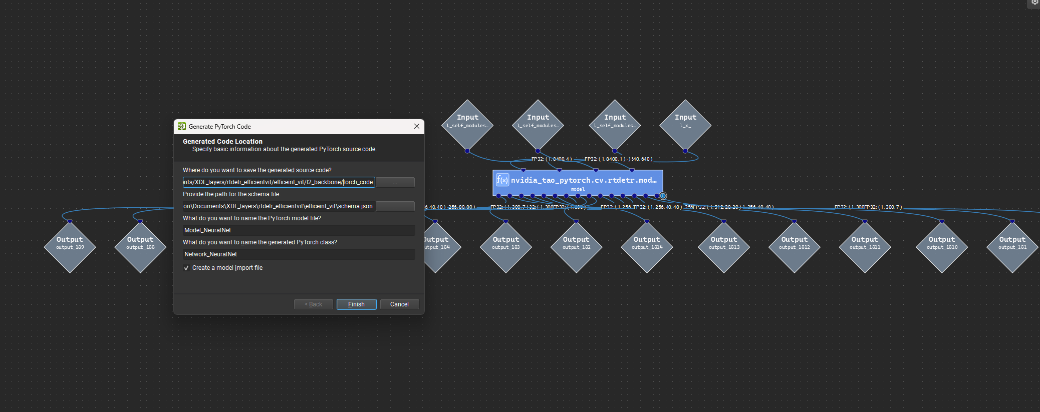
The image above shows the PyTorch export wizard for the XDL-to-PyTorch workflow.
The export wizard lets you specify:
The output folder for generated files.
The schema file used to resolve metadata during code generation.
The name of the generated PyTorch model file.
Whether to generate a companion import file.
The exporter preprocesses the active model before code generation. This preprocessing applies upgrades, expands templates, and resolves fusing-related details so the Python generator receives a flattened model description.
Requirements#
Python 3.7 or later must be available from the Nsight Deep Learning Designer process.
The schema file path must point to a valid file.
PyTorch export is available for XDL models. It is not exposed while editing templates or ONNX models.
coloramaandlarkmust be installed in either a virtual environment or the default Python environment used to run the exporter.
Generated Files#
Depending on the options you choose, export generates these files in the target folder:
The main PyTorch model file, such as
model_out.py.An optional companion import file, such as
model_out_import.py.model_support.py, which contains shared helper code used by generated models.
The generated model class derives from torch.nn.Module and implements forward(). Generated models also include a layer map so code can look up layers by their original XDL names.
If the schema describes custom plugins, the exporter can also copy the plugin’s Python implementation and referenced CUDA library into the generated output folder, then instantiate the plugin using the schema-provided script.
Command-Line Export#
The UI export command ultimately runs XDLtoPyTorch.py. You can also run that script directly:
python XDLtoPyTorch.py -f <output-folder> -p <model.py> -s <schema.json> <model.xdlm>
Useful options:
-ccreates the companion import file.-moverrides the generated PyTorch class name.-vprints tensor-size information when the generated model is first evaluated.
For example:
python XDLtoPyTorch.py -c -v -f models -p denoiser.py -m DENOISER -s schema.json denoiser.xdlm
Practical Notes#
Export is intended to generate a starting point for PyTorch training code. You are expected to add your own dataset, optimizer, loss, and training loop.
Import quality depends on whether the source
nn.Modulecan be captured as a single FX graph and whether that graph can be mapped onto supported XDL layers and parameters.Models with TorchDynamo graph breaks are not supported by the importer. See the PyTorch graph-break documentation: Working with Graph Breaks.
For custom layers or plugins, keep the related schema file with your conversion workflow so metadata can be resolved consistently in both directions.
For custom plugin export workflows, treat the importer-emitted
new_schema.jsonas a starting point and add any export-side metadata that your generated PyTorch code needs.
User Tools#
Nsight Deep Learning Designer supports custom user tools when user workflows require processing beyond what the Global Model Modification system provides. User tools are a way to incorporate custom processing of an ONNX model as part of the Nsight Deep Learning Designer design workflow.
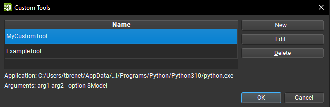
Custom tools can be managed through a dialog accessible under Tools > Custom Tools. The dialog contains a list of user-defined custom tools. Selecting a tool from the list shows its application path and arguments at the bottom. A selected custom tool can be deleted or edited using the corresponding buttons on the right side of the dialog.
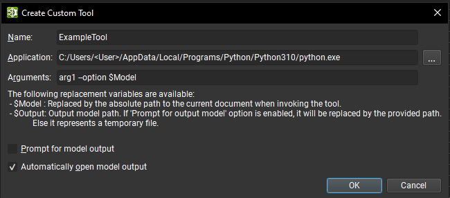
A new custom tool can be created using the Create button, this opens a new dialog window where the tools information must be provided:
A unique name used to identify the tool.
The application path representing the executable process launched to start the tool.
Optional arguments to pass to the application. Two special replacement arguments are available:
$Model: is replaced by the current ONNX document absolute path when launching the tool.$Output: is replaced by a destination file the tool should use to save the modified model. The Prompt for Model Output option prompts for this path. If the option is disabled, this is a path to a temporary file.
Prompt for model output: if turned on, when invoking the tool a dialog box opens asking for a path that is used to replace the
$Outputargument.Automatically open model output: if turned on, when the tool successfully finished and, if an
$Outputvariable was set in the argument list, Nsight Deep Learning Designer automatically opens the output document.
Note that to run a Python script, the application path should point to the Python interpreter and the first argument provided should be the path to the Python script.
Custom user tools can be found under the Tools > User Tools sub-menu, selecting a tool from that menu invokes it given the currently focused ONNX model. A dialog window opens and provides the current status of the tool process with the standard output and error logs. A custom tool process can be canceled using the Cancel button, this results in the process getting killed. Depending on whether the Automatically open model output option was set or not for the tool, Nsight Deep Learning Designer opens the output model, if any, when the tool exits successfully.
Activities Platform Settings#
Nsight Deep Learning Designer activities run on a target machine. Activities can be run locally on Linux, Windows, or NVIDIA L4T, or remotely on Linux and NVIDIA L4T target machines (from any supported Nsight Deep Learning Designer host). The Host platform refers to the the machine where Nsight Deep Learning Designer is running. And the Target platform to the machine where an activity is run. For activities run locally, the host and target machines are the same.
Connection Management#
When starting an activity in Nsight Deep Learning Designer, the top part of the activity window is used to select on which target machine the activity is performed. Both local and remote targets are supported depending on the platform type. The platform on which the host application is running is selected by default.
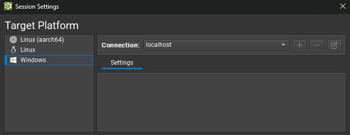
Currently Nsight Deep Learning Designer supports the following platforms:
Windows x86_64: local only.
Linux x86_64: local and remote.
NVIDIA L4T arm64: local and remote.
Linux SBSA arm64: local and remote.
When using a remote target, a Connection must be selected or created from the top drop down. To create a new connection, select + and enter the Remote Connection details. When using the local platform, localhost is selected as the default and no further connection settings are required.
Remote Connections#
Remote targets that support SSH can be configured as a target in the Connection Dialog. To configure a remote device, ensure an SSH-capable Target Platform is selected, then press the + button. The following configuration dialog is presented.
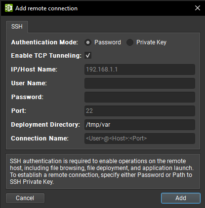
Nsight Deep Learning Designer supports both password and private key authentication methods. In this dialog, select the authentication method and enter the following information:
Password
IP/Host Name: The IP address or host name of the target device.
User Name: The user name to be used for the SSH connection.
Password: The user password to be used for the SSH connection.
Port: The port to be used for the SSH connection. (The default value is 22.)
Deployment Directory: The directory to use on the target device to deploy supporting files. The specified user must have write permissions to this location. Relative paths are supported.
Connection Name: The name of the remote connection that shows up in the Connection Dialog. If not set, it defaults to
<User>@<Host>:<Port>.
Private Key
IP/Host Name: The IP address or host name of the target device.
User Name: The user name to be used for the SSH connection.
SSH Private Key: The private key that is used to authenticate to the SSH server.
SSH Key Passphrase: The passphrase for your private key.
Port: The port to be used for the SSH connection. (The default value is 22.)
Deployment Directory: The directory to use on the target device to deploy supporting files. The specified user must have write permissions to this location. Relative paths are supported.
Connection Name: The name of the remote connection that shows up in the Connection Dialog. If not set, it defaults to
<User>@<Host>:<Port>.
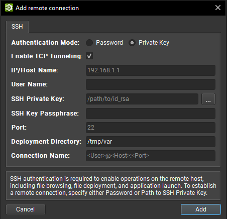
In addition to keyfiles specified by path and plain password authentication, Nsight Deep Learning Designer supports interactive authentication and standard keyfile path searching. When all information is entered, click the Add button to make use of this new connection.
Once an activity has been launched remotely, the required binaries and libraries are copied, if necessary, to the Deployment Directory on the remote machine.
On Linux and NVIDIA L4T host platforms, Nsight Deep Learning Designer supports SSH remote profiling on target machines which are not directly addressable from the machine the UI is running on through the ProxyJump and ProxyCommand SSH options. These options can be used to specify intermediate hosts to connect to or actual commands to run to obtain a socket connected to the SSH server on the target host and can be added to your SSH configuration file.
Note that for both options, Nsight Deep Learning Designer runs external commands and does not implement any mechanism to authenticate to the intermediate hosts using the credentials entered in the Connection Dialog. These credentials are only used to authenticate to the final target in the chain of machines.
When using the ProxyJump option, Nsight Deep Learning Designer uses the OpenSSH client to establish the connection to the intermediate hosts. This means that in order to use ProxyJump or ProxyCommand, a version of OpenSSH supporting these options must be installed on the host machine.
A common way to authenticate to the intermediate hosts in this case is to use an SSH agent and have it hold the private keys used for authentication.
Since the OpenSSH SSH client is used, you can also use the SSH askpass mechanism to handle these authentications in an interactive manner.
For more information about available options for the OpenSSH client and the ecosystem of tools it can be used with for authentication refer to the official manual pages.
Deployment Workflow#
Activities in Nsight Deep Learning Designer depend on shared libraries to support inference. For example, the TensorRT profiler depends on the TensorRT libraries and Nsight Systems. Nsight Deep Learning Designer uses an on-demand deployment workflow, meaning that those dependencies are not installed alongside Nsight Deep Learning Designer but are deployed on the selected target before launching an activity.
Before starting an activity, Nsight Deep Learning Designer checks if all the necessary dependencies are present on the target machine; for remote targets, Nsight Deep Learning Designer looks inside the provided Deployment Folder. A dialog shows the list of dependencies for the activity and the verification progress. If some dependencies are missing or not up to date, their entries in the dialog show a warning icon and Nsight Deep Learning Designer starts their deployment on the target.
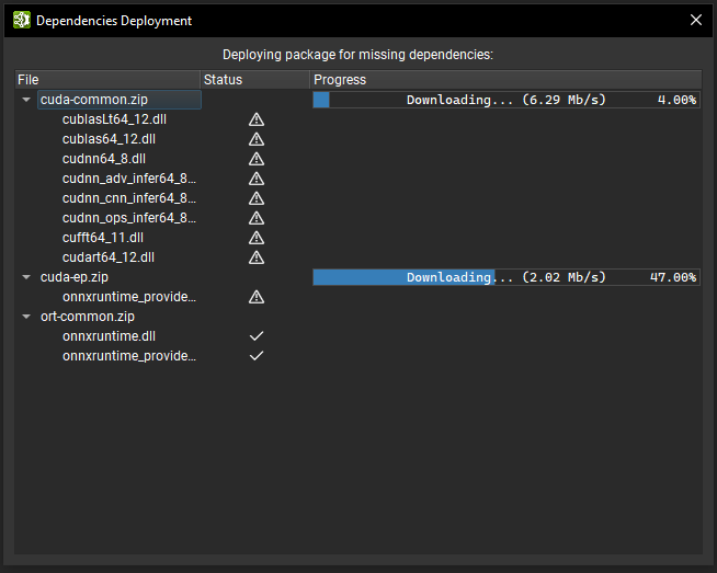
To deploy dependencies, Nsight Deep Learning Designer runs an helper binary on the target machine (deployed over SSH for remote targets) which downloads the necessary packages from a storage server over HTTPS. The helper binary then extracts the new libraries from the packages. The deployment dialog shows the progress of package downloads and the extraction process. Note that the target machine must have internet access for on-demand deployment to work.
When HTTPS deployment to a remote target fails, Nsight Deep Learning Designer proposes a fallback workflow which involves first deploying the dependencies on the local machine where the host application is running, and then transferring each dependency over SSH to the target machine. Note that this fallback workflow is expected to be slower as files that needs to be transferred are usually large (over 200 MB).
After all dependencies have been deployed on the target machine, Nsight Deep Learning Designer proceeds with the activity launch. Subsequent launches are faster as Nsight Deep Learning Designer does not redeploy dependencies as long as they still match activity requirements.
Nsight Deep Learning Designer stores downloaded dependencies and helper binaries for the target machine on the host, and stores timing caches and some other validation caches on the target machine, in a local cache directory. By default, the local cache directory is stored in $HOME\AppData\Local on Windows, and in $HOME/.config on Linux. This directory can be changed by setting the NV_DLD_CACHE_DIR environment variable.
Working with TensorRT#
Nsight Deep Learning Designer can export ONNX models to TensorRT engines and optionally profile them. The resulting engine files are fully compatible with other TensorRT applications.
Notes:
TensorRT engines created with Nsight Deep Learning Designer are specific to both the TensorRT version with which they were created and the GPU on which they were created. See the TensorRT documentation for details.
Nsight Deep Learning Designer uses a timing cache when building TensorRT networks. Tactic timings for frequently used layers will be loaded from the cache when possible.
The engine build and profiling phases rely on accurate timings of inference algorithms for engine optimization and performance reporting. For best results, do not run other GPU work in parallel with TensorRT activities, as this will skew results.
Both export and profiling activities can be launched from the Start Activity dialog accessible from the Welcome page.
Dynamic Shapes and TensorRT#
TensorRT requires an optimization profile when working with dynamic input sizes. Statically determined input sizes do not require additional information, but each dynamic input size (such as ['batch', 3, 544, 960] or ['W', 'H']) requires optimization profile details. If an input is not fully specified in this fashion, TensorRT will fail with an error such as input_name: dynamic input is missing dimensions in profile 0.
Nsight Deep Learning Designer provides two ways to define optimization profiles within the host GUI:
Dynamic inputs with a single leading wildcard (such as
['batch', 3, 544, 960],['size'], or['n', 204800, 4]) may be set automatically with a prefilled value called the Inferred Batch Size. Inputs with more than one wildcard dimension may not be defined using inferred batch sizes.Optimization profiles for individual layers can be set via the TensorRT Optimization Profile attribute. Right click on an input layer in the canvas or Layer Explorer and select the Set TensorRT Optimization Profile context menu item. This will open a dialog where you can define the minimum, maximum, and optimal sizes for the input. The optional
size-minandsize-maxfields are used to define the minimum and maximum sizes for the input. This option is recommended for detailed exploration of models with multiple wildcards. The figure below shows the optimization profile editor. Note that optimization profiles can only be applied to inputs to the top-level graph, and not to subgraphs or local functions.
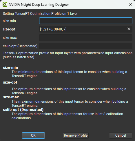
Specifying Layer Precisions to TensorRT#
Note
Layer precision constraints apply only to TensorRT 10.x.
When run with the default settings, TensorRT will use autotuning to select datatype precision for each layer from the enabled tactics to maximize performance. However, precision constraints may be enforced on a per-layer basis by use of the TensorRT Layer Precision attribute in Nsight Deep Learning Designer. The available floating-point precision options are: fp32, fp16, bf16, and fp8. The integral options are int64, int32, int8, int4, uint8, and bool. If a layer is not assigned a precision, TensorRT will use autotuning to select the best precision for that layer. Note that in addition to specifying precision constraints, you must also set the Typing Mode to Obey Precision Constraints or Prefer Precision Constraints in the activity settings. See below for more details.
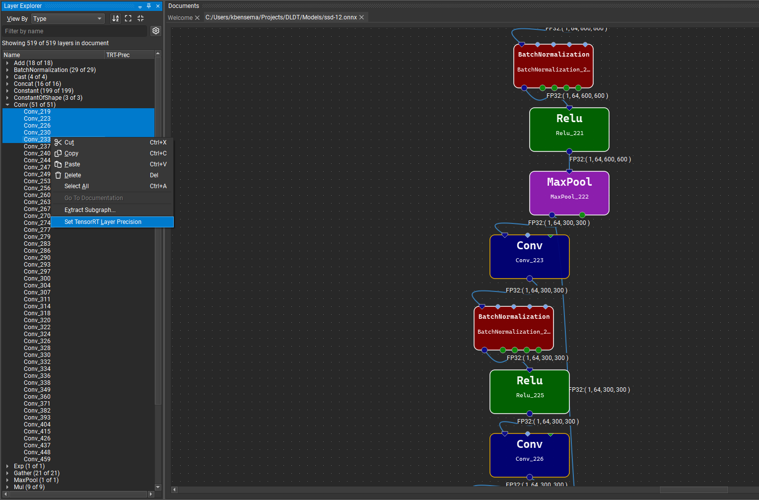
Layer precision constraints may be set in Nsight Deep Learning Designer by right-clicking selected rows in the Layer Explorer or nodes in the model canvas, and selecting the Set Layer Precision context menu item, and then selecting a precision option in the dialog that appears. To clear a precision constraint, select the No Constraint option for the selected layers.
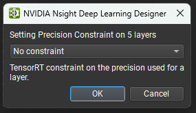
Layers with precision constraints will have the constraint value shown in the TRT-Prec column in the Layer Explorer, and a small badge with selected precision will appear on the layer glyph. Clicking this badge shows a quick menu of options to change or remove the constraint.
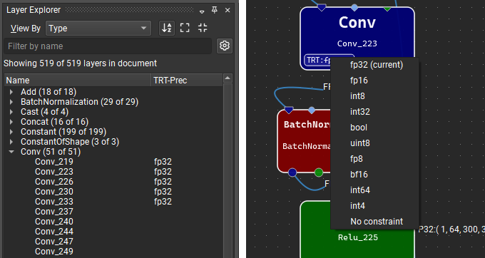
Exporting a TensorRT Engine#
To export a TensorRT engine, open the ONNX model you wish to export and use the File > Export > TensorRT Engine menu item. ONNX models can also be exported from the Start Activity dialog without opening them beforehand.
Selecting a Version#
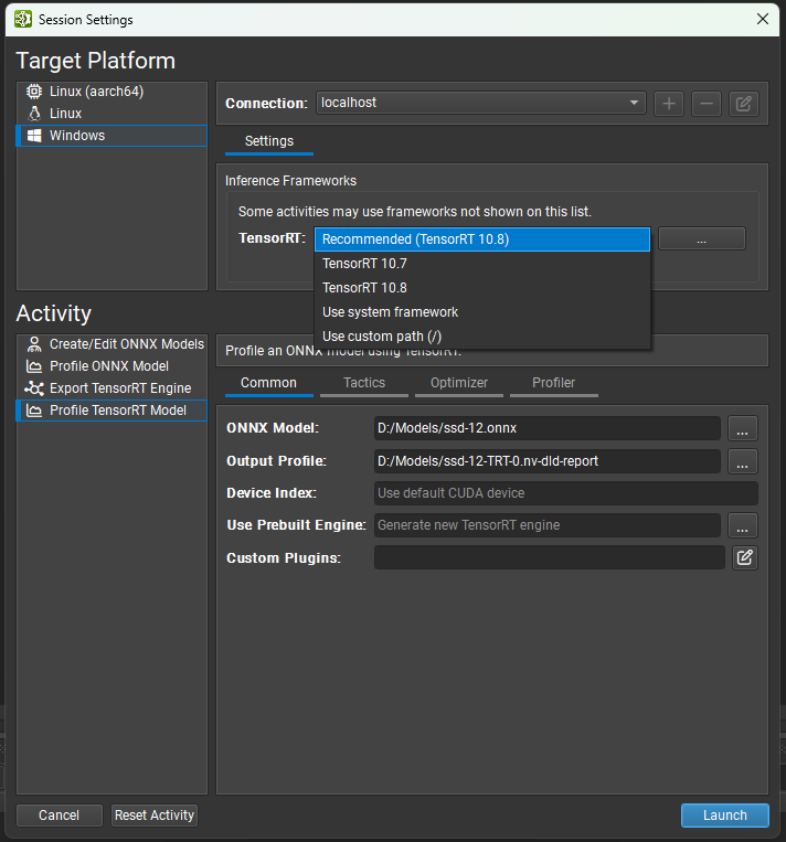
Nsight Deep Learning Designer supports multiple minor versions of TensorRT 10 and 11 for profiling. Use the dropdown selector to choose the version of TensorRT you wish to use. There are selected versions of TensorRT available for automatic download and deployment (along with a recommended version). You may also elect to use the system-installed TensorRT on the target system, or specify a custom path. If you specify a custom path, it must be a relative path from the deployment directory on the target machine to the location of the TensorRT shared libraries.
TensorRT activities in Nsight Deep Learning Designer are separated by major version since TensorRT 10.x and 11.x do not share a compatible ABI. Fields in the following sections typically apply to both TensorRT 10.x and 11.x, but will be documented if they apply to only a single framework.
Common Settings#
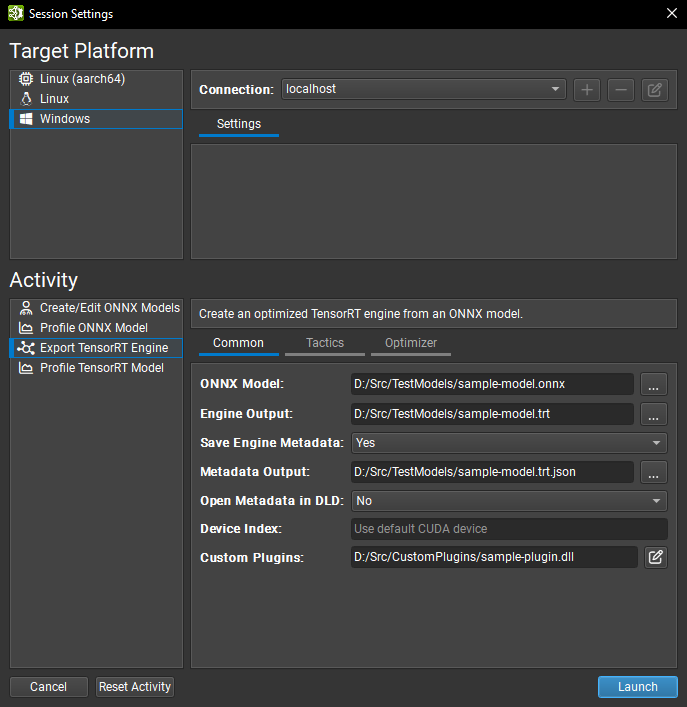
The Model Type setting controls whether you export an ONNX or XDL model. Some options may be hidden depending on the selected value.
The ONNX Model setting (ONNX only) or XDL Model setting (XDL only) is the local path to the model you wish to export. It will be copied to the target system if necessary.
The XDL Weight Atlas setting (XDL only) is the local path to the XDL model’s weight atlas. It will be copied to the target system if necessary.
The Prune Dangling Nodes setting (XDL only) controls whether XDL layers not contributing to a network output will be excluded from the ONNX export.
The Engine Output parameter is the local destination where you wish to save the exported TensorRT engine. It will be copied from the target system if necessary. The activity suggests a default name for this parameter based on the input model filename.
The Save Engine Metadata parameter controls the amount of metadata stored in the TensorRT engine. When set to Yes,
DETAILED-level metadata (full information) will be stored in the engine. Setting this option to No removes all layer information.The Metadata Output parameter is optional. If a local path is provided for this parameter, Nsight Deep Learning Designer will create an instance of the TensorRT
IEngineInspectorclass after export and copy its output from the target system. If this parameter is left blank, no metadata file will be created. The activity suggests a default name for this parameter based on the ONNX model filename.The Open Metadata in DLD parameter controls whether the metadata file is opened for visualization as a model in Nsight Deep Learning Designer after export. This option is only available if a metadata file is generated.
The Device Index option controls which CUDA device to use on multi-GPU systems. Device 0 represents the default CUDA device, and devices are ordered as in the
cudaSetDevicecall. If this setting is left blank, Nsight Deep Learning Designer will use the first CUDA device. The syntax for this field is identical to that of theCUDA_VISIBLE_DEVICESenvironment variable; see the CUDA documentation for details.The Custom Plugin parameter allows passing paths to optional custom TensorRT plugins to load during engine building. Provided paths must be relative to the selected target system. Plugins must be compatible with the selected TensorRT version. Refer to the TensorRT documentation for more details on custom plugins.
Tactics Settings#
Most settings in this section map closely to TensorRT’s BuilderFlags enumeration.
FP32 tensor formats and tactics are always available to TensorRT. TensorRT may still choose a higher-precision layer format if it results in overall lower runtime or if no lower-precision implementations exist.
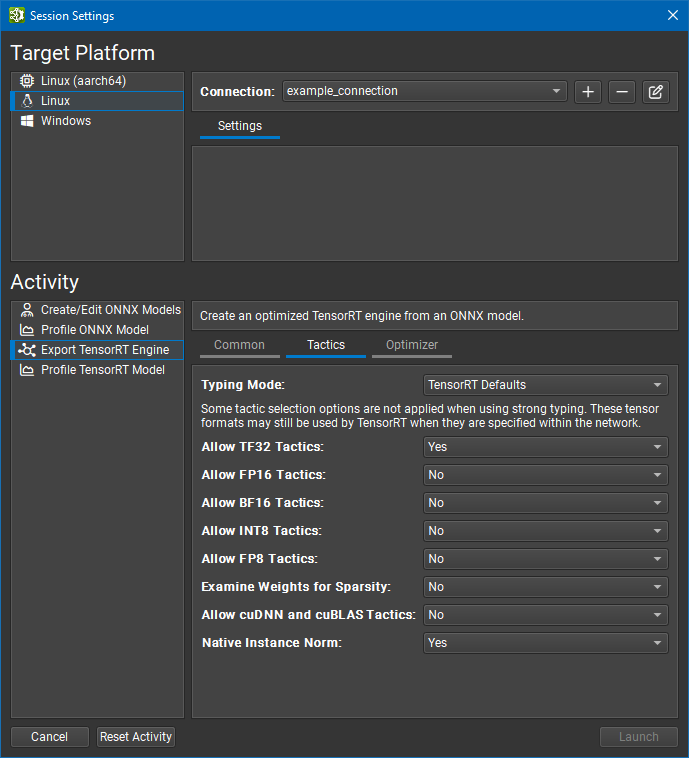
The Typing Mode setting (TensorRT 10 only) controls TensorRT’s type system:
The TensorRT Defaults option instructs TensorRT’s optimizer to use autotuning to determine tensor types. This option generates the fastest engine but can result in accuracy loss when model accuracy requires a layer to run with higher precision than what TensorRT chooses. Layer precision constraints are ignored in this mode.
The Strongly Typed option instructs TensorRT’s optimizer to determine tensor types using the rules in the ONNX operator type specification. Types are not autotuned and may result in a slower engine than one where TensorRT chooses tensor types, but the smaller set of kernel alternatives can improve the engine build time. Layer precision constraints and the FP16, BF16, INT8, and FP8 tactics settings are ignored in this mode.
The Obey Precision Constraints option uses TensorRT autotuning where layer precision constraints have not already been set using Nsight Deep Learning Designer. If no layer implementation exists for a particular precision constraint, the engine build will fail.
The Prefer Precision Constraints option is similar to Obey Precision Constraints, but TensorRT will issue warning messages instead of failing to build an engine if layer precision constraints cannot be observed or result in a slower network.
TensorRT 11 supports only strong typing.
The Allow TF32 Tactics setting allows TensorRT’s optimizer to select TensorFloat-32 precision. This format requires an NVIDIA Ampere GPU architecture or newer.
The Allow FP16 Tactics setting (TensorRT 10 only, not available with strong typing) allows TensorRT’s optimizer to select IEEE 754 half precision.
The Allow BF16 Tactics setting (TensorRT 10 only, not available with strong typing) allows TensorRT’s optimizer to select Bfloat16 precision. This format requires an NVIDIA Ampere GPU architecture or newer.
The Allow INT8 Tactics setting (TensorRT 10 only, not available with strong typing) allows TensorRT’s optimizer to use quantized eight-bit integer precision. Explicitly quantized networks are recommended, but Nsight Deep Learning Designer will assign placeholder dynamic ranges (similar to
trtexec) if the network is implicitly quantized and no calibration cache is provided.The Allow FP8 Tactics setting (TensorRT 10 only, not available with strong typing) allows TensorRT’s optimizer to use quantized eight-bit floating-point precision. This setting is mutually exclusive with the INT8 setting and is typically needed only for networks with optional FP8 tensors generated by plugins.
The Allow INT4 Tactics setting (TensorRT 10 only, not available with strong typing) allows TensorRT’s optimizer to select four-bit integer precision.
The Allow FP4 Tactics setting (TensorRT 10 only, not available with strong typing) allows TensorRT’s optimizer to select quantized four-bit floating-point precision.
The Examine Weights for Sparsity setting instructs TensorRT’s optimizer to examine weights and use optimized functions when weights have suitable sparsity.
The Strict NaNs for Sparsity setting instructs TensorRT’s optimizer to disable floating-point optimizations that might hide the generation or propagation of NaN or infinite values. This setting is typically enabled in conjection with the Examine Weights for Sparsity option described above.
Optimizer Settings#
Settings in this page primarily control the TensorRT IBuilderConfig interface.
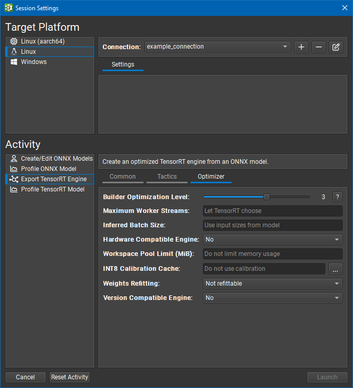
The Builder Optimization Level option controls the tradeoffs made between engine build time and inference time. Higher optimization levels allow the optimizer to spend more time searching for optimization opportunities, which may result in better performance at runtime. See the TensorRT
setBuilderOptimizationLevelfunction documentation for more details.The Maximum Worker Streams option controls multi-stream inference. If the model contains operators that can run in parallel, TensorRT can execute them on auxiliary streams. The value of this setting defines the maximum number of streams to provide to TensorRT at build time. If this setting is left blank, TensorRT will use internal heuristics to choose an appropriate number. Set this value to zero to disable stream parallelism.
The Inferred Batch Size option allows implicit specification of TensorRT optimization profiles for dynamic inputs of the form
['N', sizes...].The Hardware Compatibility Mode option creates a TensorRT engine that works on additional TensorRT-supported discrete GPUs beyond the specific GPU it was created for.
The No extra compatibility setting disables the hardware compatibility feature.
The All Ampere and later GPUs setting creates a TensorRT engine that works on all GPUs with the NVIDIA Ampere GPU architecture or newer. Use of this feature may have a performance impact as it limits shared memory usage and can preclude optimizations for later GPU architectures. Use of this feature requires an NVIDIA Ampere GPU architecture or newer.
The Same compute capability setting creates a TensorRT engine that works on all GPUs with the same CUDA Compute Capability as the GPU the engine was built on. This feature may have a performance impact. Use of this feature requires an NVIDIA Turing GPU architecture or newer.
The Workspace Pool Limit (MiB) option controls the size of the workspace memory pool used by TensorRT. The value should be specified in mibibytes; one MiB is 220 bytes. Setting this value too small may prevent TensorRT from finding a valid implementation for a layer. Leaving this value blank (the default) removes the limit and allows TensorRT to use all available global memory on the GPU.
The INT8 Calibration Cache (TensorRT 10 only) option allows you to specify a calibration cache file for implicitly quantized INT8 networks. Leaving this value blank (the default) will disable calibration. Calibration caches are neither required nor used when the network is explicitly quantized or does not enable INT8 tactics.
The Weights Refitting option controls whether weights are stored in the generated TensorRT model and whether they can be altered at inference time. The Not refittable option is the TensorRT default. It embeds weights which may not be refitted. The Refittable (Weights included) option corresponds to TensorRT’s
kREFITflag; it embeds weights and permits all weights to be refitted. The Refittable (Weights stripped) option corresponds to TensorRT’skSTRIP_PLANflag. This option embeds only those weights with performance-sensitive optimizations; all other weights are omitted and refittable. Applications are expected to refit the original weights into the engine at inference time.The Refitted Weights are Identical option allows TensorRT to assume that refit weights will be identical to those provided at build time. The resulting engine will have the same performance as a non-refittable one, but TensorRT behavior is undefined if refit weights are not identical to the build-time weights.
The Version Compatible Engine option creates a TensorRT engine that can be used for inference with later versions of TensorRT. See the TensorRT documentation for details.
Visualizing a TensorRT Engine#
The layers of a TensorRT engine can be visualized in Nsight Deep Learning Designer via the metadata file optionally generated during TensorRT engine export activities or on the command line with the trtexec tool. If generating a metadata file outside of Nsight Deep Learning Designer, the --profilingVerbosity flag must be set to detailed.
An existing TensorRT engine metadata file can be opened in Nsight Deep Learning Designer by using the File > Open menu item and selecting the metadata file. The engine will be visualized as a model in the workspace. As this is only a metadata file describing an engine; no edits to parameters or layers can be made. Note that Nsight Deep Learning Designer expects a .trt.json file extension.
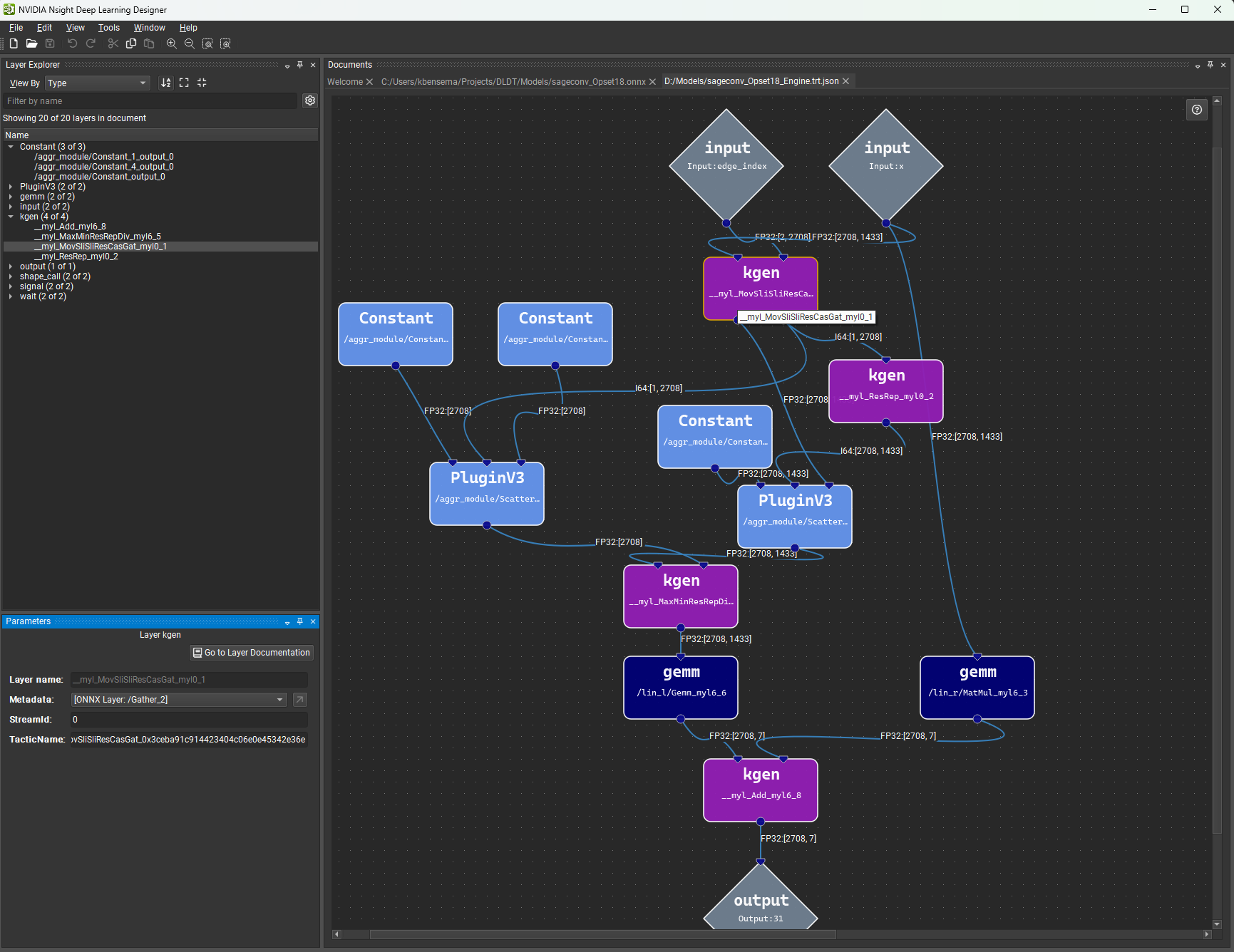
When a TensorRT kernel node has an available Metadata parameter, the user can open the source ONNX model and jump to one of the nodes that the kernel represents in the execution graph. The figure below shows the list of available source nodes to jump to in the dropdown list. The red-boxed button jumps to the selected source node. The user may have to provide a path to the ONNX source model.
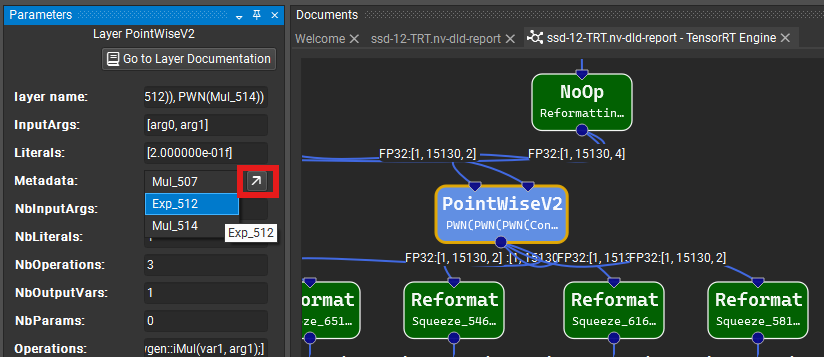
The visualization of the TensorRT engine can be customized under the TensorRT category in the Options > Model Canvas settings page. Layers may be colored by kernel type or by stream ID. Links, in addition to the default constant color, may be colored by tensor type and precision. The image below shows an example of a TensorRT engine with layers colored by kernel type and links colored by tensor type and precision.
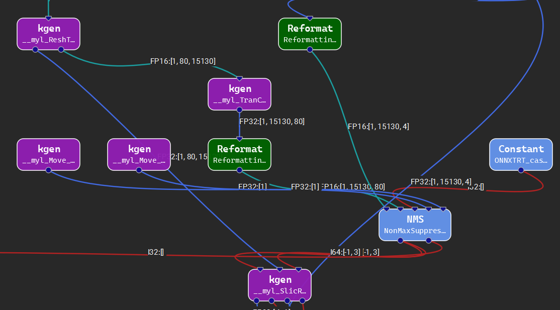
Profiling#
Nsight Deep Learning Designer supports profiling networks using either TensorRT or ONNX Runtime as the inference framework. GPU performance metrics are available only when profiling with TensorRT.
To profile, open the model you wish to profile and use the Profile Model toolbar button or Tools > Profile Model menu item. Models can also be profiled from the Start Activity dialog without opening them beforehand.
Note: When targeting the NVIDIA L4T platform, the user (local or remote) needs to be a member of the debug group in order to profile.
Profiling with ONNX Runtime#
To profile a model using ONNX Runtime, open the model you wish to profile and use the Tools > Profile Model menu item. Models can also be profiled from the Start Activity dialog (accessible through the Welcome page) without opening them beforehand.
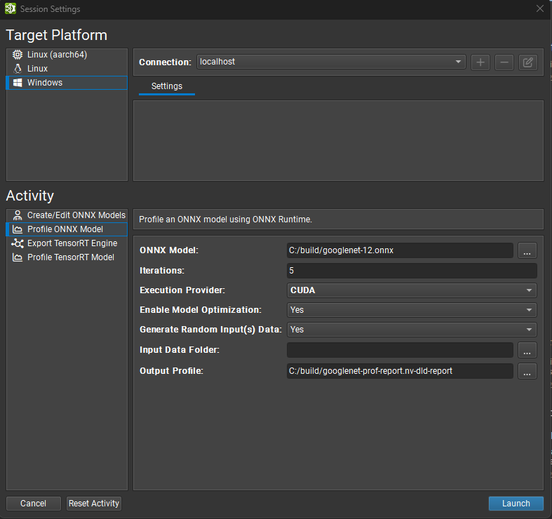
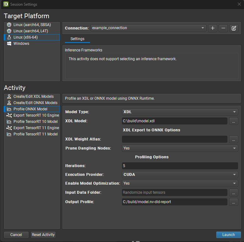
Nsight Deep Learning Designer’s ONNX Runtime profiler is based on the ONNXRuntime Performance Test binary. The options for ONNX Runtime profiling are below:
The Model Type setting controls whether you profile an ONNX or XDL model. Some options may be hidden depending on the selected value.
The ONNX Model setting (ONNX only) or XDL Model setting (XDL only) is the local path to the model you wish to profile. It will be copied to the target system if necessary.
The XDL Weight Atlas setting (XDL only) is the local path to the XDL model’s weight atlas. It will be copied to the target system if necessary.
The Prune Dangling Nodes setting (XDL only) controls whether XDL layers not contributing to a network output will be excluded from the ONNX export.
The Iterations option controls how many inference iterations are performed when gathering data. Increasing this value reduces noise when computing the median inference pass as more data points are sampled, but correspondingly increases the time taken to profile the model.
The Execution Provider option defines which backend the ONNX Runtime profiler will use during inference. The CPU and CUDA providers are supported on all target platforms. Windows targets also support the DirectML provider.
The Enable Model Optimization option controls whether the profiler should first apply graph-level transformations to optimize the model before running inference. If turned on, the profiler applies the highest level of optimization as described in Graph Optimizations in ONNX Runtime.
The Input Data Folder option controls where the profiler should find the data for the model’s input. When this entry is left blank, the profiler will generate random data for model inputs. Free dimensions are treated as 1. When not blank, this option should point to a directory containing one file with an ONNX TensorProto per model input. The Protobuf file needs to be named as its corresponding model’s input, example:
input_0.pb. The input data will be copied to the target system if necessary.The Output Profile parameter is the local destination where you wish to save the profiler report. It will be copied from the target system if necessary. The activity suggests a default name for this parameter based on the model filename.
Profiling with TensorRT#
To profile a model using TensorRT, open the model you wish to profile and use the Tools > Profile Model menu item. Models can also be profiled from the Start Activity dialog (accessible through the Welcome page) without opening them beforehand.
Profiling ONNX models with dynamic input sizes requires a TensorRT optimization profile. Input optimal sizes are used by the profiler when generating random input data.
Selecting a Version#
Nsight Deep Learning Designer supports multiple minor versions of TensorRT 10 and 11 for profiling. Use the dropdown selector to choose the version of TensorRT you wish to use. There are selected versions of TensorRT available for automatic download and deployment (along with a recommended version). You may also elect to use the system-installed TensorRT on the target system, or specify a custom path. If you specify a custom path, it must be a relative path from the deployment directory on the target machine to the location of the TensorRT shared libraries.
TensorRT activities in Nsight Deep Learning Designer are separated by major version since TensorRT 10.x and 11.x do not share a compatible ABI. Fields in the following sections typically apply to both TensorRT 10.x and 11.x, but will be documented if they apply to only a single framework.
Common Settings#
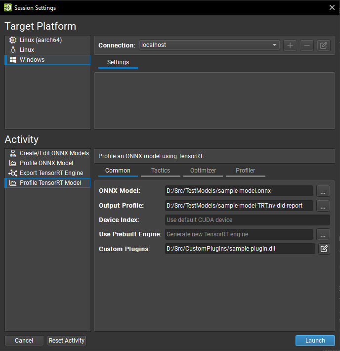
The Model Type setting controls whether you export an ONNX or XDL model. Some options may be hidden depending on the selected value.
The ONNX Model setting (ONNX only) or XDL Model setting (XDL only) is the local path to the model you wish to export. It will be copied to the target system if necessary.
The XDL Weight Atlas setting (XDL only) is the local path to the XDL model’s weight atlas. It will be copied to the target system if necessary.
The Prune Dangling Nodes setting (XDL only) controls whether XDL layers not contributing to a network output will be excluded from the ONNX export.
The Output Profile parameter is the local destination where you wish to save the profiler report. It will be copied from the target system if necessary. The activity suggests a default name for this parameter based on the model filename.
The Device Index option controls which CUDA device to use on multi-GPU systems. Device 0 represents the default CUDA device, and devices are ordered as in the
cudaSetDevicecall. If this setting is left blank, Nsight Deep Learning Designer will use the first CUDA device. The syntax for this field is identical to that of theCUDA_VISIBLE_DEVICESenvironment variable; see the CUDA documentation for details.The Use Prebuilt Engine option allows you to profile a pre-existing TensorRT engine from the Export TensorRT Engine activity or other workflows such as
trtexecinstead of building a new one. The engine file must have been built from the ONNX model being profiled, must havekDETAILEDprofiling verbosity, and will automatically be refitted before inference if possible. Settings in the Tactics and Optimizer pages are ignored when profiling a prebuilt engine. The engine is considered trusted, and any embedded host code (as by the TensorRT version compatibility or plugin embedding options) will be deserialized and executed as necessary.The Custom Plugins parameter allows passing paths to optional custom TensorRT plugins to load during engine building. Provided paths must be relative to the selected target system. Plugins must be compatible with the selected TensorRT version. Refer to the TensorRT documentation for more details on custom plugins.
The Input Data Folder option controls whether the profiler randomizes inference inputs or loads them from NumPy files. When this field is left blank (the default), inputs will be randomized as in previous versions of Nsight Deep Learning Designer. If not blank, the option must be set to the local path to a folder containing input tensors. Each input should be named
inputname.npy, where inputname is the name of a network input with nonalphanumeric characters replaced by underscores. Input tensors loaded from disk must match their corresponding TensorRT input type.Randomly generated inputs use data-type-specific distributions:
Type
Generated values
FP32, FP16, BF16
Sampled from a standard normal distribution (mean 0, variance 1), then converted to the target type.
INT32, INT64, BOOL
Uniformly distributed across the full numeric range of the type.
INT8, UINT8, INT4, FP4
Random encoded storage values across the full byte or nibble range.
FP8
Random encoded FP8 values across the non-NaN range. NaN bit patterns are replaced with zero.
The Output Data Folder option allows you to save the network outputs to disk after inference. If this option is not blank, each output will be saved to this path using the name
outputname.npy, where outputname is the name of a network output with nonalphanumeric characters replaced by underscores.
In this version of Nsight Deep Learning Designer, only the following TensorRT data types can be loaded from or saved to NumPy files: FP32, FP16, INT8, INT32, BOOL, UINT8, and INT64. Other data types, and tensor formats other than kLINEAR, are not supported within the profiler.
Tactics Settings#
Most settings in this section map closely to TensorRT’s BuilderFlags enumeration.
FP32 tensor formats and tactics are always available to TensorRT. TensorRT may still choose a higher-precision layer format if it results in overall lower runtime or if no lower-precision implementations exist.
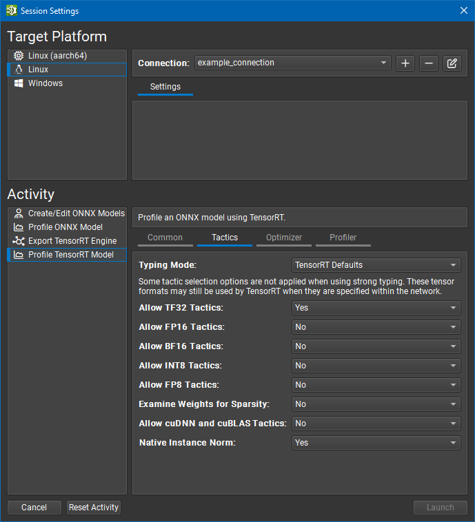
The Typing Mode setting (TensorRT 10 only) controls TensorRT’s type system:
The TensorRT Defaults option instructs TensorRT’s optimizer to use autotuning to determine tensor types. This option generates the fastest engine but can result in accuracy loss when model accuracy requires a layer to run with higher precision than what TensorRT chooses. Layer precision constraints are ignored in this mode.
The Strongly Typed option instructs TensorRT’s optimizer to determine tensor types using the rules in the ONNX operator type specification. Types are not autotuned and may result in a slower engine than one where TensorRT chooses tensor types, but the smaller set of kernel alternatives can improve the engine build time. Layer precision constraints and the FP16, BF16, INT8, and FP8 tactics settings are ignored in this mode.
The Obey Precision Constraints option uses TensorRT autotuning where layer precision constraints have not already been set using Nsight Deep Learning Designer. If no layer implementation exists for a particular precision constraint, the engine build will fail.
The Prefer Precision Constraints option is similar to Obey Precision Constraints, but TensorRT will issue warning messages instead of failing to build an engine if layer precision constraints cannot be observed or result in a slower network.
TensorRT 11 supports only strong typing.
The Allow TF32 Tactics setting allows TensorRT’s optimizer to select TensorFloat-32 precision. This format requires an NVIDIA Ampere GPU architecture or newer.
The Allow FP16 Tactics setting (TensorRT 10 only, not available with strong typing) allows TensorRT’s optimizer to select IEEE 754 half precision.
The Allow BF16 Tactics setting (TensorRT 10 only, not available with strong typing) allows TensorRT’s optimizer to select Bfloat16 precision. This format requires an NVIDIA Ampere GPU architecture or newer.
The Allow INT8 Tactics setting (TensorRT 10 only, not available with strong typing) allows TensorRT’s optimizer to use quantized eight-bit integer precision. Explicitly quantized networks are recommended, but Nsight Deep Learning Designer will assign placeholder dynamic ranges (similar to
trtexec) if the network is implicitly quantized and no calibration cache is provided.The Allow FP8 Tactics setting (TensorRT 10 only, not available with strong typing) allows TensorRT’s optimizer to use quantized eight-bit floating-point precision. This setting is mutually exclusive with the INT8 setting and is typically needed only for networks with optional FP8 tensors generated by plugins.
The Allow INT4 Tactics setting (TensorRT 10 only, not available with strong typing) allows TensorRT’s optimizer to select four-bit integer precision.
The Allow FP4 Tactics setting (TensorRT 10 only, not available with strong typing) allows TensorRT’s optimizer to select quantized four-bit floating-point precision.
The Examine Weights for Sparsity setting instructs TensorRT’s optimizer to examine weights and use optimized functions when weights have suitable sparsity.
The Strict NaNs for Sparsity setting instructs TensorRT’s optimizer to disable floating-point optimizations that might hide the generation or propagation of NaN or infinite values. This setting is typically enabled in conjection with the Examine Weights for Sparsity option described above.
Optimizer Settings#
Settings in this page primarily control the TensorRT IBuilderConfig interface.
The Builder Optimization Level option controls the tradeoffs made between engine build time and inference time. Higher optimization levels allow the optimizer to spend more time searching for optimization opportunities, which may result in better performance at runtime. See the TensorRT
setBuilderOptimizationLevelfunction documentation for more details.The Maximum Worker Streams option controls multi-stream inference. If the model contains operators that can run in parallel, TensorRT can execute them on auxiliary streams. The value of this setting defines the maximum number of streams to provide to TensorRT at build time. If this setting is left blank, TensorRT will use internal heuristics to choose an appropriate number. Set this value to zero to disable stream parallelism.
The Inferred Batch Size option allows implicit specification of TensorRT optimization profiles for dynamic inputs of the form
['N', sizes...].The Hardware Compatibility Mode option creates a TensorRT engine that works on additional TensorRT-supported discrete GPUs beyond the specific GPU it was created for.
The No extra compatibility setting disables the hardware compatibility feature.
The All Ampere and later GPUs setting creates a TensorRT engine that works on all GPUs with the NVIDIA Ampere GPU architecture or newer. Use of this feature may have a performance impact as it limits shared memory usage and can preclude optimizations for later GPU architectures. Use of this feature requires an NVIDIA Ampere GPU architecture or newer.
The Same compute capability setting creates a TensorRT engine that works on all GPUs with the same CUDA Compute Capability as the GPU the engine was built on. This feature may have a performance impact. Use of this feature requires an NVIDIA Turing GPU architecture or newer.
The Workspace Pool Limit (MiB) option controls the size of the workspace memory pool used by TensorRT. The value should be specified in mibibytes; one MiB is 220 bytes. Setting this value too small may prevent TensorRT from finding a valid implementation for a layer. Leaving this value blank (the default) removes the limit and allows TensorRT to use all available global memory on the GPU.
The INT8 Calibration Cache (TensorRT 10 only) option allows you to specify a calibration cache file for implicitly quantized INT8 networks. Leaving this value blank (the default) will disable calibration. Calibration caches are neither required nor used when the network is explicitly quantized or does not enable INT8 tactics.
The Weights Refitting option controls whether weights are stored in the generated TensorRT model and whether they can be altered at inference time. The Not refittable option is the TensorRT default. It embeds weights which may not be refitted. The Refittable (Weights included) option corresponds to TensorRT’s
kREFITflag; it embeds weights and permits all weights to be refitted. The Refittable (Weights stripped) option corresponds to TensorRT’skSTRIP_PLANflag. This option embeds only those weights with performance-sensitive optimizations; all other weights are omitted and refittable. Applications are expected to refit the original weights into the engine at inference time.The Refitted Weights are Identical option allows TensorRT to assume that refit weights will be identical to those provided at build time. The resulting engine will have the same performance as a non-refittable one, but TensorRT behavior is undefined if refit weights are not identical to the build-time weights.
The Version Compatible Engine option creates a TensorRT engine that can be used for inference with later versions of TensorRT. See the TensorRT documentation for details.
Profiler Settings#
Settings in this page control the behavior of the Nsight Deep Learning Designer profiler rather than TensorRT.
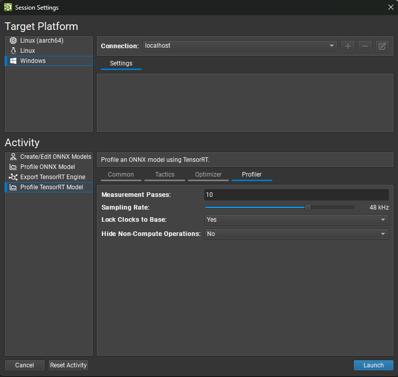
The Measurement Passes option controls how many inference iterations are performed when gathering data. Increasing this value reduces noise when computing the median inference pass as more data points are sampled, but correspondingly increases the time taken to profile the model.
The Sampling Rate option controls the frequency of GPU performance counter collection. Increasing this value collects more data for the profiling report but may overflow the collection buffer on large models.
The Hide Non-Compute Operations option controls whether to include profiler overhead such as host/device memory copies in the measurement loop and resulting profiler report.
The Collect SOC Metrics option (Linux aarch64 only) controls whether Nsight Systems should collect SOC metrics during profiling. Integrated GPU platforms such as NVIDIA Jetson should typically enable this option in order to collect memory utilization metrics, but desktop and datacenter platforms such as NVIDIA DGX Spark should disable this option as they are not SOC-based.
Non-compute operations should be hidden and the Measurement Passes value set to a large number (two hundred is usually enough) when measuring end-to-end performance in real-world configurations. Increasing the pass count ensures the GPU stays active long enough to reach its maximum clock rate. Omitting non-compute operations from the profiling operation further saturates the GPU as SM operations will not be interleaved with memory copies.
Profiling from the Command Line#
Nsight Deep Learning Designer includes a command-line profiler that supports TensorRT for non-interactive use cases. The command-line profiler is called DLDesignerWorker. It can be found in the remote or local target’s deployment directory after interactively profiling from the Nsight Deep Learning Designer GUI.
Use the profile-trtX subcommand (where X is the major TensorRT version being targeted) to profile a model with TensorRT. Full details on the command-line arguments accepted by the profiler can be viewed using the --help option. All options from the Profile TensorRT Model activity interface are supported when using the command-line profiler.
It is not necessary to save a full profiling report when using the command-line profiler. By passing the --summary command-line option (enabled by default), the profiler will display performance triage information on stdout.
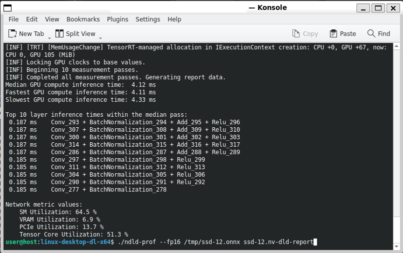
Example output from the command-line profiler#
Profiling Reports#
Nsight Deep Learning Designer uses a common report format to store profiling data from ONNX Runtime and TensorRT. Existing profiling reports can be reopened using the File > Open File command. The Profile TensorRT Model and Profile ONNX Model activities will automatically open the new profiler report upon a successful profiling run.
The profiling report describes the execution of the ONNX model (or the one exported from an XDL model) as performed by the selected inference framework, which typically refers to a runtime-optimized version of the network. Groups of nodes from the ONNX model may be fused together into single optimized layers, and other nodes may be removed entirely during an optimization pass.
Profiling reports have four major sections. Each section is described below, including any differences between the ONNX Runtime and TensorRT profilers.
Network Summary#

The summary section shows high-level details about the profiling run.
Network Name: The name of the ONNX model that was profiled, or “xdl-export” for XDL models.
Backend: The inference framework used for profiling, whether ONNX Runtime or TensorRT.
Execution Provider (ONNX Runtime only): The preferred ONNX Runtime execution provider used for profiling.
Inference Device (TensorRT only): The name of the GPU used for inference, as returned by the CUDA driver.
Profiler Version (TensorRT only): The version of Nsight Deep Learning Designer used to create the profiler report.
Nsight Systems Version (TensorRT only): The version of Nsight Systems used to create the profiler report.
Median Network Inference Time: The elapsed wall clock time taken by the median inference pass.
# Inference Passes: The number of inference passes performed during profiling.
Device Memory Required (TensorRT only): The maximum device memory required by the compiled TensorRT engine during inference, as returned by
ICudaEngine::getDeviceMemorySize.Serialized Engine Size (TensorRT only): The size of the generated TensorRT engine as it would be stored on disk.
Model Weights Size (TensorRT only): The size of the model weights stored within the TensorRT engine. For engines built with the
kSTRIP_PLANflag (“weightless” engines), this field additionally shows the stripped weight size.
Inference Timeline#
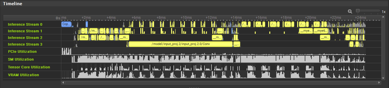
The inference timeline shows the execution of the individual layers within the median inference pass. Each concurrent stream of execution (as in TensorRT’s multi-stream inference feature) is shown in a separate row. The view can be scrolled using the scrollbar and zoomed by holding Ctrl while moving the mouse wheel. Specific time durations may be measured by clicking the left mouse button and dragging. Additional zoom options are available through a context menu, accessed by clicking the right mouse button within the timeline.
TensorRT only: Overhead from host-to-device (H2D) input copies and device-to-host (D2H) output copies is included in the timeline.
Layers identifiable as “overhead,” such as reformat operations, memory copies, and TensorRT NoOp layers, are depicted in the timeline using a different color from normal computation layers.
GPU Metrics (TensorRT only)#
The Nsight Deep Learning Designer TensorRT profiler collects GPU-level performance metrics during inference. These metrics are displayed as extra rows within the timeline. Values are normalized for rendering in order to fill the available vertical space; hover the mouse cursor over a data point to see the actual value collected.
SMs Active: Fraction of time where at least one warp was executing on the streaming multiprocessor (SM). Heavy utilization of the SM is associated with compute-bound operations.
DRAM Throughput: Fraction of peak throughput of the GPU DRAM controller. Heavy utilization of the DRAM controller is associated with memory-bound operations on the GPU.
PCIe Throughput: Fraction of peak throughput of the PCI Express bus. Heavy utilization of the PCIe bus is associated with memory copies between the CPU and GPU.
Tensor Active: Fraction of time where the SM’s tensor cores were active. Heavy utilization of SM tensor cores indicates the inference framework performed significant work with reduced-precision tensor formats.
Compute Warps in Flight: Fraction of peak throughput of compute shader warps. High throughput of compute warps indicates the GPU pipelines are fully saturated.
Network Metrics and Layer Table#
The Network Metrics section provides a detailed view of individual layers’ execution behavior within the inference framework.

The summary view shows the most common values for each column of the table. When multiple values appear for a discrete variable such as Precision or Input Dimensions, the full list of values remains accessible. Hovering the mouse cursor over the list will show a tooltip with every observed value in descending order of frequency. Continuous variables such as inference time are presented as minimum, maximum, total, and average (arithmetic mean) values.
When selecting multiple layer rows, the summary view changes to reflect the selected layers. If only a single layer is selected, or the selection is cleared, the summary view returns to showing the entire inference pass.
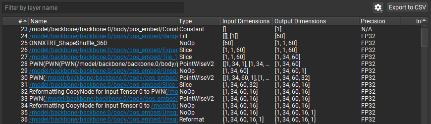
The layer table displays information on each layer of the executed network. This table can be exported to CSV format using the Export to CSV button. The Open Model button displays a menu of related models to open. Options are the ONNX source model, and if profiling with TensorRT, the metadata for the TensorRT engine that was profiled. Typing into the Filter by layer name text box filters the table to only those layers which contain the filter text as a substring. The filtering check is case-insensitive.
The Settings button (displayed as a gear) displays a popup menu with options for the layer table:
Show Inference Time Heat Colors renders inference time columns using a color scale such that longer-executing layers appear in a more intense color. Multiple color schemes are available. The color scale can be changed from the Environment tab of the Options dialog, accessible using Tools > Options.
Use Full Pass Time in Percentages controls how inference time percentages are calculated. By default, which is the unchecked state, layer inference time percentages are relative to the sum of individual layer inference times, hiding framework overhead such as input buffer copies. When this setting is checked, layer inference time percentages are instead calculated relative to the duration of the entire inference pass.
Each layer of the executed network is displayed as a separate row in the table. Double-clicking an entry in the table zooms the timeline to fit the layer within view. This layer table contains the following information columns:
#: The inference order of each layer. For multi-stream inference, the order reflects when a layer is enqueued to a stream, not necessarily when it begins executing.
Name: The name of the layer. Many optimized layer names contain information about their originating ONNX nodes. Clicking a hyperlink within the layer will open the original ONNX model within the Nsight Deep Learning Designer editor and select the corresponding node. Clicking the magnifying glass button for a selected layer will pop up a menu of associated ONNX source nodes: those nodes contributing directly to the optimized layer, those nodes which generated the input tensors consumed by the optimized layer, and those nodes which consumed outputs from the optimized layer. Selecting any of those options within the menu will open the source ONNX model and select the node as though clicking a hyperlink.
Type: The type of the layer as reported by the inference framework.
Input Dimensions: The dimensions of the layer’s input tensors.
Output Dimensions: The dimensions of the layer’s output tensors.
Execution Provider (ONNX Runtime only): The ONNX Runtime execution provider used for this layer.
Precision: The input precision of this layer. For layers with multiple inputs, this is the precision of the first input tensor. Layers with no direct input tensors, such as Constant layers, are shown here as
N/A.Inference Time (%): The inference time of this layer represented as a percentage. See Use Full Pass Time in Percentages for a description of how this percentage is calculated.
Inference Time (ms): The inference time of this layer in milliseconds.
Layer Table Hierarchy (TensorRT only)#
The Nsight Deep Learning Designer TensorRT profiler keeps track of the layer hierarchy within the source ONNX model. When possible, TensorRT profiler reports will show that hierarchy in the layer table.
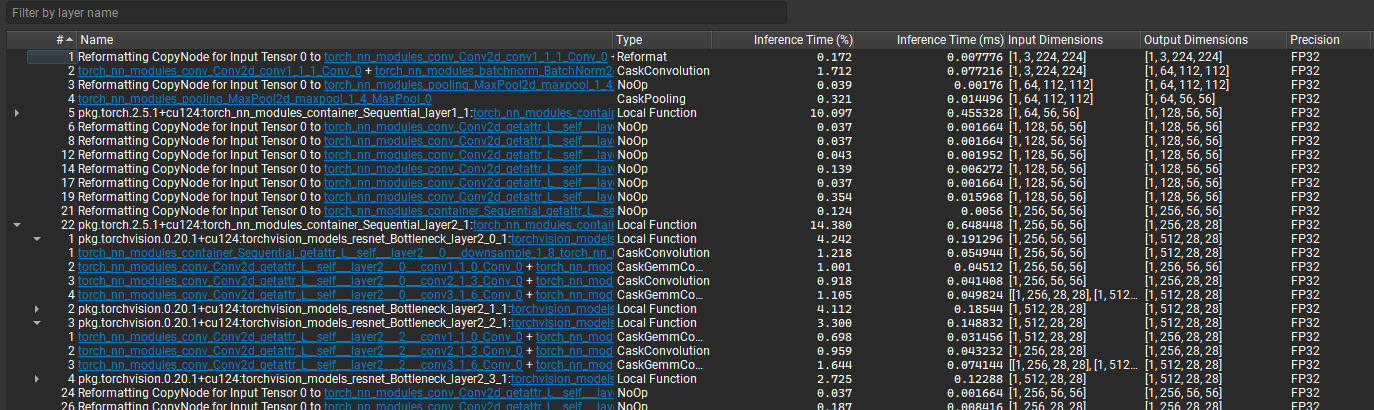
Layers that are part of an ONNX local function or subgraph are grouped under an expandable entry in the layer table representing that local function or subgraph instance. Note that TensorRT might inline ONNX local functions or subgraphs before profiling, in that case Nsight Deep Learning Designer is not able to show the hierarchy in the layer table. Children layers are sorted by their execution order during inferencing.
Selecting a local function or subgraph entry in the layer table will automatically select all of its children.
The parent’s reported inference time is the sum of its child layers’ inference times within the inference stream. If the child layers were enqueued across multiple inference streams, the value shown is the maximum time spent in a single stream.
The parent’s displayed input dimensions and precision are those of the first child layer it executed. Similarly, the output dimensions of the parent are those of the final child layer it executed.
Network Graphs#
The profiler report includes two graphs summarizing layer behavior by type. These graphs can be resized by dragging the splitter that separates them from the layer table.
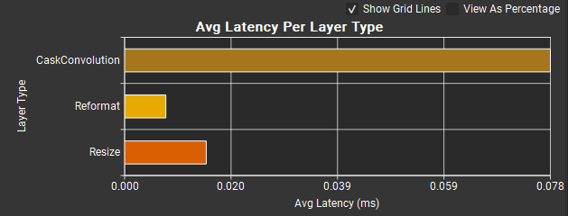
The Average Latency per Layer Type graph displays the average inference time for each layer type in the network. Longer bars represent longer inference times. The horizontal axis scale is in milliseconds by default. Checking the View as Percentage checkbox will rescale the X axis to represent percentages of the summed layer inference times. The Use Full Pass Time in Percentages option described earlier does not apply to this graph.
The Show Grid Lines checkbox controls whether grid lines are displayed within the graph.
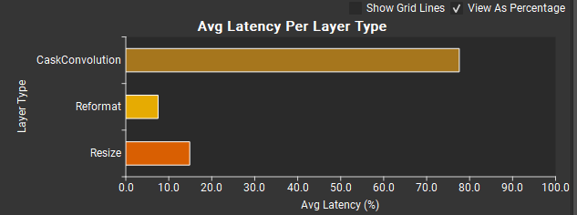
The previous graph, but with View as Percentage checked and Show Grid Lines unchecked.#
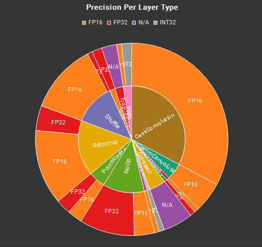
The Precision per Layer Type graph displays the distribution of input tensor precisions used for each layer type. The inner ring of the pie chart contains the various layer types executed by the network. Each layer type is subdivided in the outer ring by its instance precisions as defined in the layer table. In the example above, all CaskConvolution layers executed in FP16 precision but the PointWiseV2 layers executed in an equal mix of FP16 and FP32 precision. Layers executing in FP32 represent an opportunity to reduce precision for improvements in memory footprint and execution performance.
Networks with many operator types may result in small individual segments within the chart. Hover the mouse over a graph segment to explode it visually and display a tooltip with the segment’s text and value. Layer type percentages (the inner ring of the graph) are relative to the total number of layers within the network. Layer precision percentages (the outer ring) are relative to the number of layers of that type.
Working with TAO Deploy#
Warning
This feature is deprecated and will be removed in a future release of Nsight Deep Learning Designer.
Nsight Deep Learning Designer integrates with the NVIDIA TAO Deploy framework to generate TensorRT engines from TAO-derived ONNX models and optionally profile them.
Both of these activities can be launched from the Start Activity dialog. If already editing the ONNX model inside the Nsight Deep Learning Designer editor, this dialog can also be launched from the Profile Model toolbar button or Tools > Profile Model menu item.
Before Starting the Activity#
NVIDIA TAO has an installation procedure separate from that of Nsight Deep Learning Designer. We recommend setting up the TAO target machine independently before launching TAO activities with Nsight Deep Learning Designer.
Target Setup#
Install the NVIDIA TAO launcher on an x86-64 Linux machine following the directions in the TAO Toolkit Getting Started Guide.
Configure a
~/.tao_mounts.jsonfile on the target machine following the instructions in the TAO Launcher documentation.Ensure the TAO Deploy container can be started and can access the GPU. This may be done by activating the TAO Python environment and then launching the container with
tao deploy model_agnostic run nvidia-smi.
Nsight Deep Learning Designer Setup#
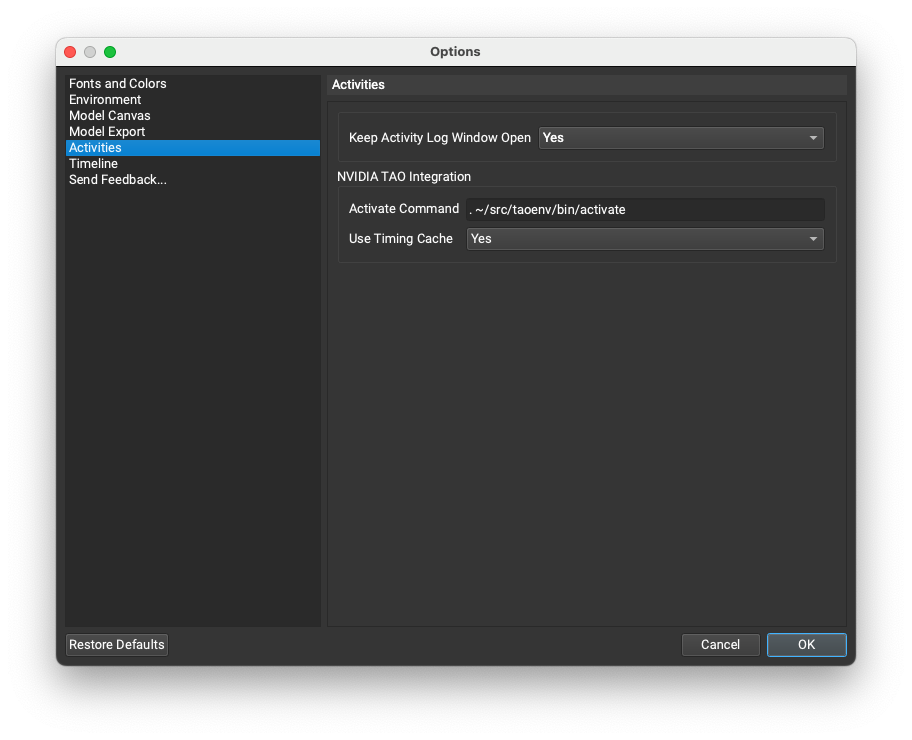
Paste the Python environment activation command used for your TAO environment into the Nsight Deep Learning Designer options dialog under Activities > NVIDIA TAO Integration > Activate Command.
This activation command is provided directly to the shell and typically requires sourcing a script.
Conda-like environments can be activated using the Miniconda install path:
source /path/to/miniconda/bin/activate environment_nameVirtualenv-like environments have individual activation scripts:
source /path/to/environment_name/bin/activate
Warning
Nsight Deep Learning Designer does not launch an interactive shell for TAO activities. Conda auto-initialization hooks in .bashrc will generally not execute, requiring use of an explicit activate script instead of the friendlier conda activate alias.
By default, Nsight Deep Learning Designer uses a persistent TensorRT timing cache to speed up TensorRT engine builds. To disable use of the timing cache, set Activities > NVIDIA TAO Integration > Use Timing Cache to No.
Experiment Setup#
Pretrained ONNX models compatible with the NVIDIA TAO framework are available from the TAO Model Zoo. You can also export TAO models from training checkpoints using the tao model <model_name> export task; see the model-specific TAO documentation for additional details on the export process.
Nsight Deep Learning Designer relies on experiment specification files when launching NVIDIA TAO activities; these are not generated from within Nsight Deep Learning Designer and should be supplied from your own TAO workflows. See TAO Deploy Modelwise Instructions for details on experiment specs for individual models. If you are a new user of TAO we recommend following the TAO tutorials; these notebooks include sample experiment specs.
Warning
Nsight Deep Learning Designer uses the model_agnostic TAO entry point and therefore relies on the model architecture to be provided inside the experiment specification file. Be sure that the experiment spec YAML contains an appropriate model_name entry. As a general rule, the model_name for a model is the subcommand used in the TAO CLI, such as dino for DINO, rtdetr for RT-DETR, or visualchangenet for VisualChangeNet.
Filesystem paths within the experiment spec are in the container filesystem namespace, not the target’s filesystem namespace. Container mount points are defined in the ~/.tao_mounts.json file. Nsight Deep Learning Designer mounts additional directories within the container when executing activities. We recommend treating the /mnt/dld_*/... prefixes as reserved and not mounting your own filesystems within these directories.
Model settings defined in Nsight Deep Learning Designer typically override those defined in the experiment spec; leaving an optional setting blank in the activity configuration dialog will usually delegate it to the value from the experiment spec. See the setting description in this user guide for details on which YAML field it corresponds to.
TAO activity launches in Nsight Deep Learning Designer will include experiment.yaml files in the results directory. These files are merged experiment specs reflecting both the original TAO experiment definition and all overrides applied by Nsight Deep Learning Designer. They are provided both for later reference and as a potential baseline for future experiments.
Deploy TAO Model#
The Deploy TAO Model activity generates a TensorRT engine from an ONNX file using the TAO framework and corresponding experiment spec. This activity corresponds to the TAO Deploy gen_trt_engine task.
Common Settings#
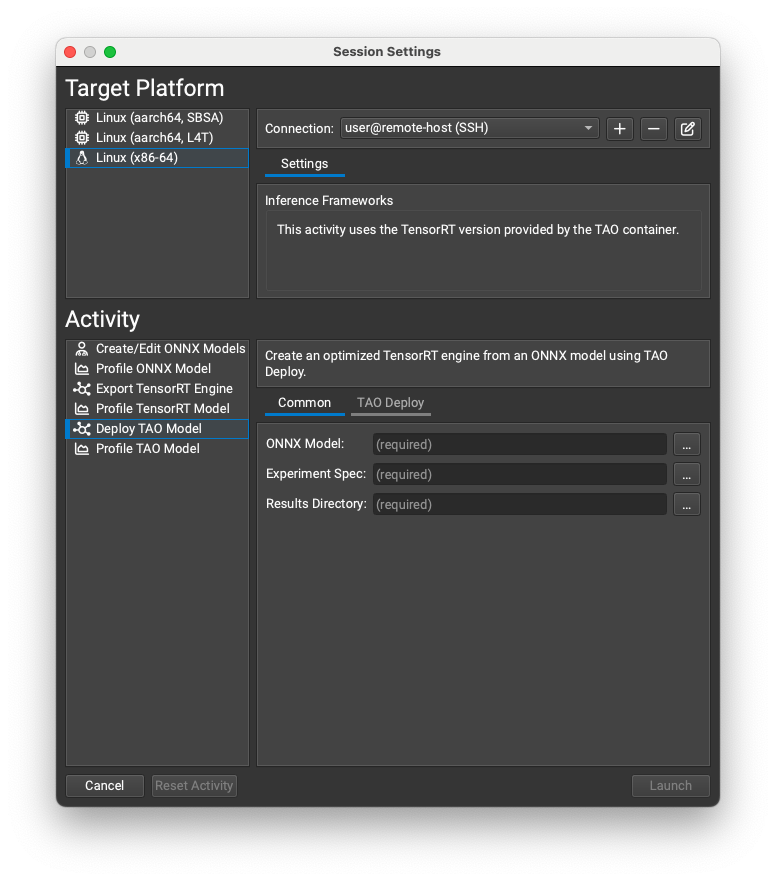
The ONNX Model parameter is the local path to the model you wish to deploy. It will be copied to the target system if necessary.
The Experiment Spec parameter is the local path to the model experiment spec. It will be copied to the target system if necessary.
The Results Directory parameter is the local destination where you wish to save the activity results.
Upon completion of the activity, the results directory will contain the following files:
gen_trt_engine.log: Standard output from the TAO engine generation task as captured bytee.gen_trt_engine/experiment.yaml: Merged experiment specification containing the original experiment YAML as modified by Nsight Deep Learning Designer model and activity settings.gen_trt_engine/status.json: Output log file as generated by the TAO framework.gen_trt_engine/tao_engine.trt: The generated TensorRT engine file.
TAO Deploy Settings#
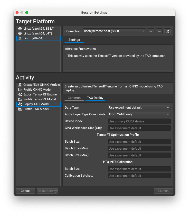
This activity settings page provides quick access to common TAO engine generation options.
The Data Type parameter selects the tensor precision to be used for the TensorRT engine. Supported values include FP32, FP16, and INT8. When set to
Use experiment default, the tensor precision is taken from the experiment spec.- The Apply Layer Type Constraints parameter determines how to use the layer precision constraint feature in Nsight Deep Learning Designer. There are three possible values for this setting:
From YAML onlyignores the Nsight Deep Learning Designer layer precision constraints. Only layer constraints expressed in the experiment spec will be applied to the generated TensorRT engine.From DLD onlyapplies only those layer precision constraints defined in Nsight Deep Learning Designer. Layer constraints expressed in the experiment spec are ignored.Merge YAML and DLDapplies layer precision constraints from both Nsight Deep Learning Designer and the experiment spec. Conflicting constraints are resolved using values from Nsight Deep Learning Designer.
The Device Index parameter controls which target GPU is used for the activity. The setting may safely be left blank for single-GPU targets or multi-GPU target systems where the default CUDA device is the desired GPU. To choose a different GPU, specify its numeric index. The device numbering scheme is the same as that used by cudaSetDevice.
The GPU Workspace Size (GB) parameter constrains the workspace memory used by TensorRT. This setting may be left blank to delegate the choice to the experiment spec or (if not present in the experiment) to the TAO default value for the model architecture.
TensorRT optimization profiles for TAO activities can be controlled from either the experiment spec or this activity settings page.
Warning
TensorRT optimization profiles defined in the Nsight Deep Learning Designer ONNX editor are ignored when launching TAO activities. The gen_trt_engine workflow in TAO currently supports only batch size controls, not generic optimization profiles.
The Batch Size parameter defines the optimum batch size for the TensorRT engine. Leave it blank to use the value in the experiment spec.
The Batch Size (Min) parmeter defines the minimum batch size for the TensorRT engine. Leave it blank to use the value in the experiment spec.
The Batch Size (Max) parameter defines the maximum batch size for the TensorRT engine. Leave it blank to use the value in the experiment spec.
Nsight Deep Learning Designer also supports some of the INT8 calibration features used by TAO and TensorRT for post-training quantization.
The Batch Size parameter defines the batch size used during calibration. Leave it blank to use the value in the experiment spec.
The Calibration Batches parameter determines how many batches are used for calibration. Leave it blank to use the value in the experiment spec.
The activity settings on this page map to the following experiment parameters in the spec file:
Setting Name |
Experiment Parameter |
|---|---|
Data Type |
|
Apply Layer Type Constraints |
|
Device Index |
|
GPU Workspace Size (GB) |
|
Batch Size |
|
Batch Size (Min) |
|
Batch Size (Max) |
|
Batch Size (INT8 calibration) |
|
Calibration Batches |
|
Profile TAO Model#
The Profile TAO Model activity profiles TensorRT engines generated by the TAO gen_trt_engine activity.
By default this activity generates a fresh TensorRT engine as though executing the Deploy TAO Model activity. This feature provides rapid performance feedback when tweaking engine generation parameters such as model precisions and batch sizes. If incremental adjustment of TAO engine build parameters is not necessary, you can also provide a prebuilt engine file to the activity. Prebuilt engines reduce accidental variance (the engine file is a known constant) and, by skipping the engine build step for profiler launches, improve execution time for the activity.
Common Settings#
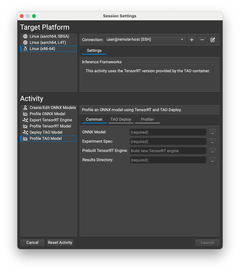
The ONNX Model parameter is the local path to the model you wish to deploy. It will be copied to the target system if necessary. This field is required even when using prebuilt engines.
The Experiment Spec parameter is the local path to the model experiment spec. It will be copied to the target system if necessary.
The Prebuilt TensorRT Engine parameter is the local path to a prebuilt TensorRT engine for the ONNX model and experiment spec. It will be copied to the target system if necessary. This field is optional; if left blank a new TensorRT engine will be generated for profiling.
The Results Directory parameter is the local destination where you wish to save the activity results.
Upon completion of the activity, the results directory will contain the following files:
gen_trt_engine.log: Standard output from the TAO engine generation task as captured bytee.gen_trt_engine/experiment.yaml: Merged experiment specification containing the original experiment YAML as modified by Nsight Deep Learning Designer model and activity settings.gen_trt_engine/status.json: Output log file as generated by the TAO framework.gen_trt_engine/tao_engine.trt: The TensorRT engine file that was used for profiling.tao_report.nv-dld-report: The profiling report.
The profiling report will be opened automatically in Nsight Deep Learning Designer upon successful completion of the activity. See Profiling Reports for more information on the TensorRT profiling report features supported by Nsight Deep Learning Designer.
TAO Deploy Settings#
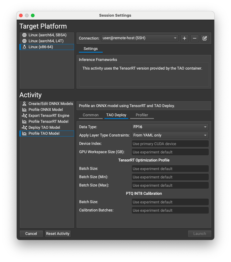
See TAO Deploy Settings for details on these options.
Note
All fields on this tab except Device Index are ignored when using prebuilt engines.
Profiler Settings#
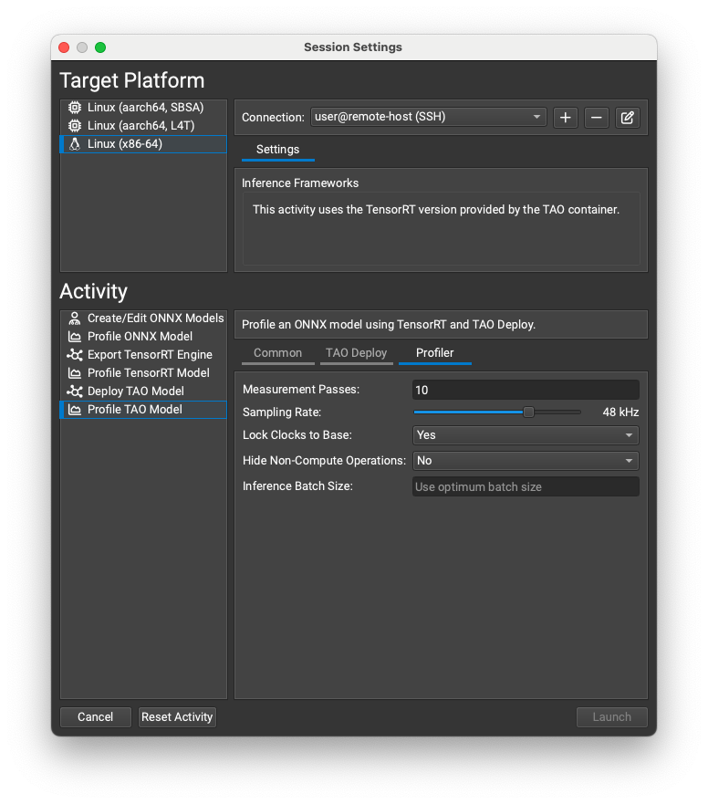
These settings control the TensorRT profiler in Nsight Deep Learning Designer. They act equivalently to the settings in the Profile TensorRT Model activity, which are also described in Profiler Settings:
The Measurement Passes option controls how many inference iterations are performed when gathering data. Increasing this value reduces noise when computing the median inference pass as more data points are sampled, but correspondingly increases the time taken to profile the model.
The Sampling Rate option controls the frequency of GPU performance counter collection. Increasing this value collects more data for the profiling report but may overflow the collection buffer on large models.
The Hide Non-Compute Operations option controls whether to include profiler overhead such as host/device memory copies in the measurement loop and resulting profiler report.
The Inference Batch Size parameter controls the batch size used for profiling. If this parameter is left blank, the profiler will use the optimum batch size used to build the TensorRT engine. The inference batch size must lie within the closed interval defined by the minimum and maximum batch sizes used to build the TensorRT engine.
Main Menu and Toolbar#
Information on the main menu and toolbar.
Editing Mode#

Main Toolbar#
The main toolbar shows commonly used operations from the main menu. See Main Menu for their description. In addition, the toolbar contains the following commands:
Profile Model
Open the most recently used Profiling activity dialog.