HydroGraphNet: Interpretable Physics-Informed Graph Neural Networks for Flood Forecasting#
HydroGraphNet is a physics-informed graph neural network for large-scale flood dynamics modeling. It integrates physical consistency, autoregressive forecasting, and interpretability through Kolmogorov–Arnold Networks (KANs) to deliver accurate and explainable predictions of water depth and volume during flooding events.
Problem Overview#
Floods, driven by climate-induced hydrologic extremes, pose significant risks to communities and infrastructure. Accurate and timely flood forecasts are critical for early warning systems and resilience planning. However, traditional hydrodynamic models, based on solving the shallow water equations, are computationally expensive and unsuitable for real-time forecasting.
HydroGraphNet addresses this challenge by offering a fast, physically consistent, and interpretable surrogate model using Graph Neural Networks. It leverages unstructured spatial meshes and incorporates physical constraints to maintain mass balance without the overhead of automatic differentiation.
Model Overview and Architecture#
HydroGraphNet#
HydroGraphNet uses an autoregressive encoder-processor-decoder GNN architecture to predict water depth and volume across multiple future time steps. The architecture comprises:
Encoder: Initializes node and edge features from spatial and hydrologic inputs.
Processor: A multi-layer message-passing network that refines node and edge features.
Decoder: Outputs the predicted changes in depth and volume, which are added to the previous state using residual connections.
The model integrates:
Physics-informed loss: Ensures mass conservation using volume continuity inequalities.
Pushforward trick: Reduces autoregressive error propagation.
Kolmogorov–Arnold Networks (KAN): Enhances model interpretability by replacing MLPs with spline-based function networks.
The training and inference pipelines use node features that include both static (e.g., elevation, slope, roughness) and dynamic (e.g., water depth, volume history) attributes, along with global forcings such as inflow hydrograph and precipitation.
Dataset#
HydroGraphNet is validated on a real-world case study from the White River near Muncie, Indiana. The dataset consists of:’
A spatial graph of 4,787 nodes,
Boundary inflow conditions and rainfall time series,
Ground truth water depth and volume over time from high-fidelity HEC-RAS simulations.
The graph representation allows flexible modeling of both fluvial and pluvial flood dynamics across urban and rural terrains.
Training the Model#
To train HydroGraphNet:
Prepare your dataset following the graph-based structure used in
HydroGraphDataset.Configure training parameters in
conf/config.yaml.Run the training script:
python train.py --config-path conf --config-name config
Training logs, model checkpoints, and metrics will be saved in the directory specified in
config.yaml.
Running Inference#
To perform autoregressive rollout and generate evaluation animations:
Configure your inference settings in
conf/config.yaml.Run the inference script:
python inference.py --config-path conf --config-name config
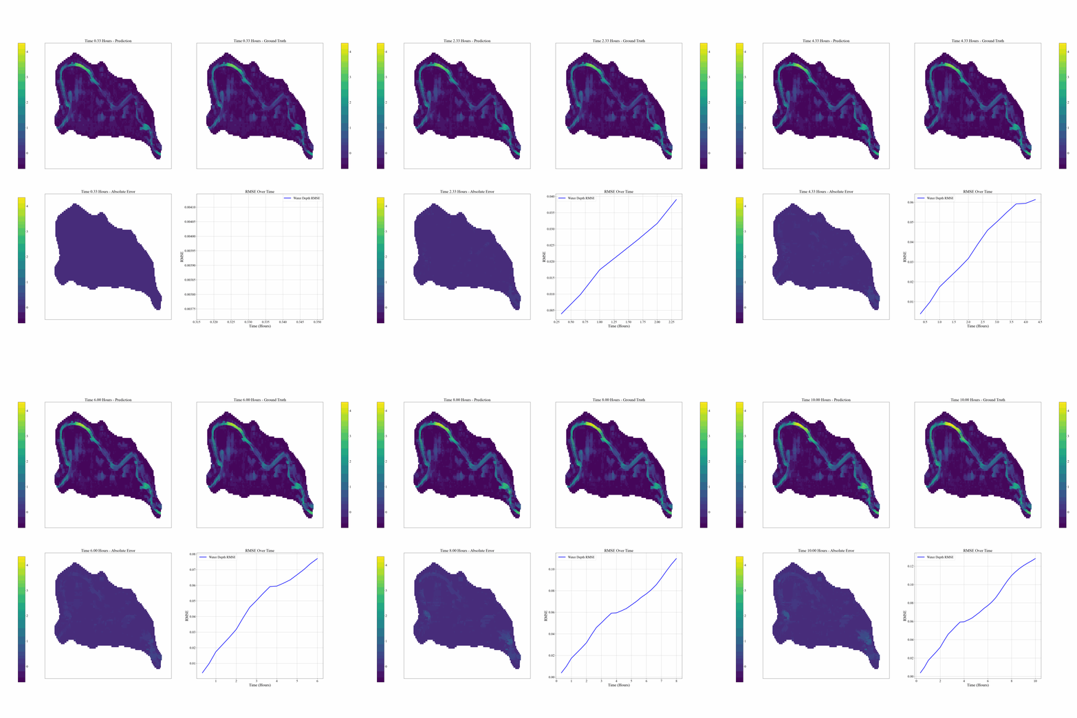
The script will output a four-panel GIF animation per test sample showing:
Predicted water depth
Ground truth water depth
Absolute error
RMSE over time

Flood Forecasting Animation#
Dataset Loading#
The dataset is handled via a custom HydroGraphDataset class, defined in hydrographnet_dataset.py. This class inherits from DGLDataset and performs the following:
Automatic downloading: If data is not available in the
data_dir, it will automatically be downloaded from Zenodo.Graph construction: Constructs a spatial graph using k-nearest neighbors over node coordinates.
Static and dynamic features: Loads and normalizes both spatial attributes (e.g., slope, curvature) and temporal inputs (e.g., water depth, precipitation).
Training mode: Returns sliding window graph samples with optional physics-aware targets.
Test mode: Returns a full graph and a rollout dictionary for inference.
To use the dataset, simply instantiate:
from hydrographnet_dataset import HydroGraphDataset

dataset = HydroGraphDataset(
    data_dir="./data",
    prefix="M80",
    split="train",  # or "test"
    n_time_steps=2,
    return_physics=True
)
This will ensure the data is downloaded, normalized, and ready for GNN training or evaluation.
Logging#
HydroGraphNet supports logging via Weights & Biases (W&B):
Training and validation losses
Physics-based loss contributions
Learning rate schedule
Set up W&B by modifying wandb_mode and watch_model in config.yaml.
Citation#
If you use HydroGraphNet in your research, please cite:
@article{taghizadeh2025hydrographnet,
  title     = {Interpretable Physics-Informed Graph Neural Networks for Flood Forecasting},
  author    = {Taghizadeh, Mehdi and Zandsalimi, Zanko and Nabian,
  Mohammad Amin and Shafiee-Jood, Majid and Alemazkoor, Negin},
  journal   = {Computer-Aided Civil and Infrastructure Engineering},
  year      = {2025},
  volume    = {n/a},
  number    = {n/a},
  pages     = {1--21},
  doi       = {10.1111/mice.13484},
  publisher = {Wiley Periodicals LLC on behalf of the Editor},
  url       = {https://onlinelibrary.wiley.com/doi/10.1111/mice.13484}
}
Contact#
For questions, feedback, or collaborations:
Mehdi Taghizadeh – jrj6wm@virginia.edu
Negin Alemazkoor – na7fp@virginia.edu