Changelog
Revision |
Date |
Changes |
|---|---|---|
| 1.0.0 | 4/19/2024 | First release |
The Aerial Omniverse Digital Twin consists of the following components:
User interface
ClickHouse
Omniverse Nucleus
Scene importer
RAN digital twin interconnected as illustrated in the following figure.
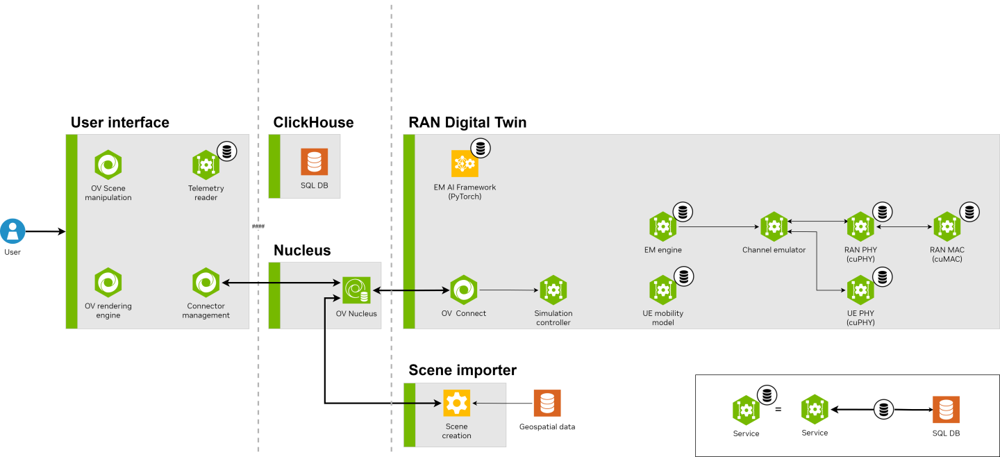
User interface
The graphical interface offers the possibility of visualizing and interacting with the scenario, as well as parametrizing, starting, interrupting and stopping simulations.
ClickHouse
The results produced by the Aerial Omniverse Digital Twin are stored in an SQL database hosted by the ClickHouse server. Correspondingly, they can be access through ClickHouse clients.
Nucleus
The Nucleus server delivers message brokering services and provisions the scene geometry to the other components. In all cases, the Nucleus server needs to be on a node whose IP address can be reached by the other components. This requires having the ports described here open.
Scene importer
The Nucleus server stores and distributes the scene geometry in the OpenUSD format. The scene importer takes in geospatial data in CityGML format and creates the OpenUSD assets needed by the Nucleus server to represent a given scene.
RAN digital twin
The actual radio access network (RAN) digital twin is in charge of
updating the positions of a population of terminals,
scheduling the transmission of data from all of the deployed radio units to all of the terminals,
computing the channel frequency response for all of the links - where a link is here intended as a wireless connection between two antenna elements - described in the scene under investigation,
generating the waveforms at the transmission point of every link,
applying the calculated frequency response, interference and noise to said waveforms, thus creating the final signal observed at the reception point of every link,
applying the necessary signal processing to extract and decode the transmitted data.
Aerial Omniverse Digital Twin (AODT) can be installed in the cloud or on-prem. The installation and operation of AODT involves deploying a set of frontend components and a set of backend components. The frontend components require one NVIDIA GPU, and the backend components require another NVIDIA GPU. The frontend components and backend components can be deployed to either the same node (i.e., colocated) or to separate nodes (i.e. multi-node). The following table details the GPU requirements for each case:
System Type |
GPU Qnty |
GPU Driver |
GPU vRAM |
GPU Requirement |
GPU Notes |
|---|---|---|---|---|---|
| Frontend alone | 1 | r535+ | 12GB+ | GTX/RTX | e.g. RTX 6000 Ada, A10, L40 |
| Backend alone | 1 | r535+ | 48GB+ | e.g. RTX 6000 Ada, A100, H100, L40 | |
| Frontend and backend colocated | 2 | r535+ | see note | see note | 1x frontend-capable GPU, 1x backend GPU |
The following table describes the OS support for each type:
System Type |
OS |
|---|---|
| Frontend alone | Windows 11, Windows Server 2022, Ubuntu 22.04 |
| Backend alone | Ubuntu 22.04 |
| Frontend and backend colocated | Ubuntu 22.04 |
For memory and CPU requirements, we recommend looking at the qualified systems in the next section.
The AODT Installer is a way to get up and running quickly with fresh installations on qualified systems, both in the cloud and on-prem. There are several components that must be installed and configured in order for a deployed system to run AODT. This section will detail how to use the AODT Installer on each of the qualified system configurations. Following those instructions will be more general guidelines to help with installations for other system configurations.
Qualified deployment targets
The following qualified systems have been tested and are directly supported with the AODT Installer:
Qualified system |
Node 1 |
Node 2 |
|---|---|---|
| Azure VM (Multi-Node) |
|
|
| Dell R750 (Colocated) |
|
N/A |
Note that Azure installations on A10 VMs require NVIDIA GRID drivers.
Azure deployment
The Aerial Omniverse Digital Twin (AODT) can be installed on Microsoft Azure using the Azure Installer. The Azure Installer in turn can be downloaded from NGC - Aerial Omniverse DT Installer using version tag 1.0.0.
Specifically, we will first download the files from the Azure folder into a local directory. In that directory, we will create a file called .secrets and define the following environment variables:
            RESOURCEGROUP=
WINDOWS_PASSWORD=
SSH_KEY_NAME=
LOCAL_IP=
GUI_OS=
NGC_CLI_API_KEY=
Variable |
Description |
|---|---|
| RESOURCEGROUP | Microsoft Azure Resource Group |
| SSH_KEY_NAME | Name of SSH key stored in Microsoft Azure |
| WINDOWS_PASSWORD | Password length must be between 12 and 72 characters and satisfy 3 of the following conditions: 1 lower case character, 1 upper case character, 1 number and 1 special character |
| LOCAL_IP | IP address (as seen by Azure) of the host that will run the provisioning scripts |
| GUI_OS | Windows |
| NGC_CLI_API_KEY | NGC API KEY |
More information on NGC_CLI_API_KEY can be found here: NGC - User’s Guide.
Also, if necessary, the following command can be used to find the external IP address of the local machine.
curl ifconfig.me
Once the variables above are configured, we can use the mcr.microsoft.com/azure-cli docker image to run the provisioning scripts.
docker run -it --env-file .secrets -v .:/aodt -v ~/.ssh/azure.pem:/root/.ssh/id_rsa mcr.microsoft.com/azure-cli
The docker container will mounts the downloaded scripts, and it will access to the private SSH key. In the example, the private key can be found in ~/.ssh/azure.pem.
Inside the docker container, we can run the following commands:
            $ az login
$ cd aodt
$ bash azure_install.sh
and the script will create the VMs, configure the network inbound ports, and download the scripts needed in the next step.
At the end, azure_install.sh will show:
            Use Microsoft Remote Desktop Connection to connect to <ip-address>
Username: aerial
Password: <configured password>
Logging into the Azure VM
We can use Microsoft Remote Desktop Client to connect to the IP address shown at the end of azure_install.sh using the configured username and password.
Once successfully logged, we can then
sign into NVIDIA Omniverse and complete the installation of the Omniverse launcher
open File Explorer, navigate to
C:\AerialODT, right clickdownload_installerand selectRun with PowerShell.
When the command is finished, we can open a Command Prompt and type
            cd c:\AerialODT
install_script.bat
At the end, the installation script will open a Jupyter notebook in the browser. We can then click on the Library tab in the Omniverse Launcher Window, and Launch the Aerial Omnivere Digital Twin graphical user interface.
Dell R750 deployment
For a full deployment on prem, we can select the pre-qualified Dell PowerEdge R750 server. After installing Ubuntu-22.04.3 Server, we can log in using SSH and run the following commands
            sudo apt-get install -y jq unzip

export NGC_CLI_API_KEY=<NGC_CLI_API_KEY>
AUTH_URL="https://authn.nvidia.com/token?service=ngc&scope=group/ngc:esee5uzbruax&group/ngc:esee5uzbruax/"

TOKEN=$(curl -s -u "\$oauthtoken":"$NGC_CLI_API_KEY" -H "Accept:application/json" "$AUTH_URL" | jq -r '.token')

versionTag="1.0.0"
downloadedZip="$HOME/aodt_bundle.zip"

curl -L "https://api.ngc.nvidia.com/v2/org/esee5uzbruax/resources/aodt-installer/versions/$versionTag/files/aodt_bundle.zip" -H "Authorization: Bearer$TOKEN" -H "Content-Type: application/json" -o $downloadedZip

# Unzip the downloaded file
unzip -o $downloadedZip
Again, more information on NGC_CLI_API_KEY can be found here: NGC - User’s Guide.
Once the aodt_bundle.zip has been downloaded and extracted, we will continue by running the following command
./aodt_bundle/install.sh localhost $NGC_CLI_API_KEY
When the installation is complete, we can use a VNC client to connect to the VNC server on port 5901. The VNC password is nvidia.
We will then sign into NVIDIA Omniverse and complete the installation in the Omniverse Launcher as for Azure. As before, a Jupyter notebook will also be opened in the browser. We can then click on the Library tab in the Omniverse Launcher Window, and Launch the Aerial Omniverse Digital Twin graphical user interface.
Validation

Once the Aerial Omniverse Digital Twin graphical interface is running, we can click on the toolbar icon showing the gears and connect to the RAN digital twin.
If asked for credentials, we can use the following:
username:
omniversepassword:
aerial_123456

Once successfully logged in, we can then select the Content tab (refer to the Graphical User Interface section for further details) and click Add New Connection. In the dialog window, we can then
type
omniverse-serverclick
OKexpand the
omniverse-servertree viewand double click on
omniverse://omniverse-server/Users/aerial/plateau/tokyo.usd

This will open the Tokyo.usd map. Once loaded, we will continue by
selecting the Viewport tab
right clicking on the Stage widget
and selecting Aerial > Create Panel twice from the context menu.
The first panel will be used - by default - for the user equipment UE and the second for the radio unit (RU).

With the panels defined, we then can
right click in the Viewport
select Aerial > Deploy RU from the context menu
and click on the final location where we would like to place the RU


With the RU is deployed, we will then select it from the Stage widget and enable the Show Raypaths checkbox from the Property widget.

Similarly, we will
right click on the Viewport
and select Aerial > Deploy UE from the context menu.
Differently from the procedure for the RU, however, this will drop the UE in the location where the right click took place.

Finally, we can
select the Scenario entry in the Stage widget
set
Duration equal to 10.0
Interval to 0.1

click the Generate UEs icon in the toolbar

click the Start UE Mobility icon
This will start a simulation and update the graphical interface as in the figure below.

By clicking on the Play button in the toolbar, we can then inspect the evolution of the mobility of the UE and the corresponding rays that illustrate how the radiation emitted by the RU reaches the UE.
The graphical user interface is illustrated in the following figure and is composed of the following elements.

1. Viewport tab
The viewport displays the geospatial data that make up the scenario and is used to deploy the radio access network (RAN) nodes or specific user equipment (UE). E.g., the deployment of a radio unit can be performed by right clicking on a given area of the map and selecting Aerial > Deploy RU from the context menu. To move the RU, once it has been selected, we can instead use Aerial > Move RU. Similarly, to manually deploy a UE, we can use Aerial > Deploy UE. (Procedural deployment of the UEs is illustrated in the simulation section).
At the top of the viewport, we can also find the settings to change the view type (e.g., top or perspective) or viewport resolution.
Finally, the color bar provides the gradient describing the power carried by each individual ray traced by the EM engine, and can be hidden or shown using CTRL+B.
2. Configuration tab
The configuration tab is used to set up the simulation and offers the following fields.

db_host: specifies the IP address of the ClickHouse server.
db_port: indicates the ClickHouse client port. By default, this field is 9000, unless ClickHouse has been installed with non-standard settings. Once db_host and db_port are specified, the user can connect to the ClickHouse server using the Connect button. If the connection is successful, the indicator next to the button will go from red to green.
db_name: this is the name of the database that will be used to store the results generated during the simulation.
db_author: this field records the author of the database. By default, it is the user ID.
db_notes: any additional text that the user intends to add to the database. This field can be left empty.
nucleus_url: the URL for the Omniverse Nucleus server.
nucleus_bc: the name of the Nucleus broadcast channel. This is the channel over which the graphical interface will search for an available worker to perform the RAN simulation.
ls_session: the name of the live session. This field can be changed in order to import or discard a given RAN deployment on the same scene.
ru_url: the URL to the 3D asset used to indicate a radio unit.
ue_url: the URL to the 3D asset used to indicate a UE.
panel_url: the URL to the asset used to express an antenna planar array.
sz_url: the URL to the asset used to indicate zone in which UEs can be procedurally spawned.
mat_url: the URL pointing to the asset that describes the ITU P.2040 materials used within the scope of the simulation.
3. Content tab
The content tab can be used to browse the content of the Nucleus server, move/copy files and open the desired scene.
4. Antenna elements tab
The antenna tab is used while setting up the simulation to specify
the type of antennas that a given antenna panel is composed of
the geometrical and polarimetric properties of said panel.
The fields of the tab are illustrated in the following figure.

panel_asset: this field specifies which panel is being edited through the tab.
antenna_type: when a given antenna site in the panel is selected, it is possible to change the type of antennas installed at the specific site. This can be done through the list of antennas found at the Antenna combo box. Once a specific antenna type is selected, it can be applied using the Apply button. If the action is successful, the field ant_type under the selected antenna sites is changed to the value indicated in the Antenna combo box. For a given site, there could be at most two colocated antennas of different polarization. This can be manipulated through the Dual Polarized check box in the property widget.
panel_sh: this field represents the uniform horizontal spacing used in the planar antenna array.
panel_sv: correspondingly, this other field indicates the uniform vertical spacing.
panel_cf: this field is in the property widget, and indicates the center frequency for which the antenna array has been designed.
panel_nh: the number of elements in a row of the planar antenna array.
panel_vh: the number of elements in a column of the planar antenna array.
panel_erf: this field expresses the roll angle, with respect to the vertical axis, of the first element in a dual polarized antenna site.
panel_ers: the corresponding roll angle for the second element in a dual polarized antenna site.
In the tab we also find two plots:
the gain pattern for the azimuthal cut
and the gain pattern for the zenithal cut
which, for the antenna type selected from the Antenna combo box, illustrate the contour of the radiation solid along the azimuthal and zenithal planes.
Finally, it is worth mentioning that the selection of a given antenna site through the left click of the mouse is additive, i.e., once a site is selected, a second one can also be added, and then a third, and so on. A second click on the selected site, will deselect it. Alternatively, the button Clear Selected can be used in order to remove any selection.
5. Console tab
This tab is used to illustrate all warnings and messages collected during the operation of the Aerial Omniverse Digital Twin. Warnings are marked in yellow, and errors are marked in red. Error of consequence for the simulation are also propagated to a dialog box.
6. Stage and property widget
The stage widget shows all the assets deployed in the scene and the property widget is the interface for setting their attributes:
Environment
This entry in the stage widget can be used to set how the scene looks and feels. It allows - for instance - to set the time of the day at the simulated location, with direct consequences on sun illumination.
Looks
This entry, if present, contains the textures used to describe the buildings.
Materials
This entry is used to list the material used across the simulation. Each material is characterized by a tuple \(\left(a,b,c,d\right)\) of four parameters, so that the relative permittivity of the material is expressed as
\( \epsilon_r = a f_{\rm{GHz}}^b - j c f_{\rm{GHz}}^d \)
as described in ITU P.2040.
Panels
This entry collects the antenna arrays used across the simulation. A new type can be added with a right click on the stage widget area and selecting Aerial > Create Panel. Once a panel is selected under this entry, we can set:
Antenna Element Type: by pressing the Edit button, we can go to the Antenna Elements tab and select one of the following antenna types:
isotropic (point source radiating in all directions with the same intensity and phase).
infinitesimal dipole
half-wave dipole
microstrip patch: reference patch antenna with
\(\epsilon_r=4.8\)
\(L = \dfrac{\lambda}{2 \sqrt{\epsilon_r}}\) (\(\lambda\) being the wavelength of the carrier)
\(W = 1.5 L\)
user input: this points to the possibility of using
Dual Polarized: this flag indicates whether the panel uses antenna arrays with dual-polarized elements.
Carrier Frequency: the center frequency at which the antenna in the array will operate.
Horizontal Elements (\(N_{hor.}\)): number of elements in a row of the planar antenna array.
Vertical Elements: (\(N_{vert.}\)): number of elements in a column of the planar antenna array.
Horizontal Spacing (\(\Delta_{hor.}\)): distance between antenna elements along each row of the planar antenna array.
Vertical Spacing (\(\Delta_{vert.}\)): distance between antenna elements along each column of the planar antenna array.
Roll of First Pol. Element: angular displacement of the element realizing the first polarization (e.g., \(45^\circ\))
Roll of Second Pol. Element: angular displacement of the element realizing the second polarization (e.g., \(-45^\circ\)). Has an effect only when the array is composed of dual polarized elements.
runtime
After they have been generated, this entry collects the trajectories along which the UEs will move during the simulation.
RUs
This entry in the stage widget collects the deployed RUs, which are added to the scene by right clicking on the viewport area with mouse and selecting Aerial > Deploy RU. By selecting a given RU in the list, we can set two different sets of properties:
Aerial Properties
Cell ID: the unique identifier that defines the cell supported by the given RU.
Panel Type: the specific antenna array for the RU currently selected.
Waveform FFT size: the size of the FFT used in a potential waveform. This parameter is used when Enable Wideband CFRs or Simulate RAN are on in Scenario.
Sub-carrier Spacing: parameter indicating the spectral distance between adjacent sub-carriers in the OFDM waveform used by the RU.
Mechanical Azimuth (\(\phi_b\)): azimuth of the RU boresight (indicated as \(\hat{b}\) in the figure below).
Mechanical Tilt (\(\theta_b\)): elevation of the RU boresight (indicated as \(\hat{b}\) in the figure below) with respect to the horizon.
Radiated power: the total radiated power, across the whole antenna array, for the given RU.
Ray Properties
Show Rays: this flag indicates whether the rays shot from a given RU needs to be included in the telemetry visualized after the simulation.

Scenario
This entry in the stage widget collects all the simulation parameters that can be currently set. This includes:
Default UE panel: this is the antenna array associated by default to any UE in the simulation. As we will see later, this parameter can be overridden locally for any given UE. This parameter is offered for convenience to programmatically associate an antenna array type to large populations of UEs.
Default RU panel: same concept as described for the default UE panel, but for the RU panel.
Enable Temperature Color: this flag indicates whether the rays need to be colored based on their relative power.
Max dynamic range: the power range in dB that should be considered for the visualization of the simulations. This range sets the power threshold - from the strongest ray - under which the graphical interface will omit the visualization of rays.
# of emitted rays (in thousands): this is the number of emitted rays at a given RU, since the rays are all traced from the RUs.
# of scene interactions per ray: the total number of admissible scattering events along any of the traced rays.
Max # of Shown Paths per RU-UE pair: this field sets the number of visualized rays per RU-UE pair.
Ray sparsity: whereas the RAN digital twin calculates the rays for all temporal samples, this field allows to only propagate a fraction of such rays to the graphical interface. This is convenient when running long simulations, which would require the transfer of substantial amount of data towards the graphical interface host, which will have to keep the data in RAM. E.g., a Ray sparsity factor of 10 means that the graphical interface will only request the rays once every 10 samples.
Batches: the number of UE redrop events during the simulation. This parameter is useful when training neural networks: in lack of aggressive parametrization of the Interval field described below, the evolution of the UEs movement is smooth and gradual. Correspondingly, the statistics of the channel does not change appreciable if not across many samples. Thanks to this parameter, it is possible to accelerate the convergence of the training process by means of UE redropping, which occur for every batch.
Enabled Wideband CFRs: this flag indicates whether channel frequency responses are also going to be generated.
Number of UEs: this indicates how many UEs will be present during the simulation. Currently limited to a maximum of 2000.
UE Height: this is the default UE height, which will be applied to all UEs in the scene.
UE Max speed: the maximum speed of the UEs in the simulation.
UE Min speed: the minimum speed of the UEs during the simulation. The actual speed of given UE will be picked from a uniform distribution going from UE Min speed to UE Max speed.
Seeded mobility: indicates whether the random number generators involved in the creation of UE mobility are seeded or not.
Seed: in case the previous parameter is set to true, this indicates the seed for the random number generators.
Enable training: this flag indicates whether we want to train a neural network while running our simulation. This is currently only supported when the RAN is not being simulated.
Simulate RAN: enables the possibility of simulating the behavior of the deployed RUs by adding a physical layer and a medium access control layer to both RUs and UEs.
Simulation mode: when Simulate RAN is disabled, this field allows to choose between two different ways of specifying the simulation timeline. In Slots mode, the simulation timeline is described by the number of slots per batch and the number of realizations of the channel per slot (Samples per slot). Differently, in Duration mode, the timeline is described by a total temporal length of simulation (Duration) and the sampling period across said duration is set by Interval. If Simulate RAN is enabled, only Slot mode is possible.
Slots per batch: number of slots to simulate for every batch in the simulation. The total number of batches in the simulation is specified in Batches.
Samples per slot: number of samples to consider in a given slot. This field can either be 1 or 14, indicating whether or not the simulation should account for the Doppler effect.
Duration: this number represents the amount of simulated time for which we would like to generate realizations of the radio environment.
Interval: this parameter indicates the sampling period with which the radio environment is to be sampled.
UEs
Once a UE is deployed, using either the viewport context menu (Aerial > Deploy UE) or the programmatic approach described next, the UE will be found under the scope of this entry. By selecting a given UE, we can configure two different sets of properties:
Aerial Properties:
User ID: the unique identifier that distinguishes a given UE from the others.
Panel Type: the specific antenna array for the UE currently selected.
Mechanical Tilt (\(\theta_b\)): elevation of the UE boresight (indicated as \(\hat{b}\) in the figure below) with respect to the horizon.
Radiated power: the total radiated power, across the whole antenna array, for the given UE.
Manually created: this flag indicates whether UE has been positioned directly by the user, or it has been generated procedurally by the software.
Ray Properties:
Show Rays from: this field indicate the list of the RUs whose rays will be included in the UE-specific telemetry visualized after the simulation.

World
This entry contains the geometry describing the scene.
7. Layer widget
The layer widget provides an alternative visualization of how the scene is composed and tracks the changes introduced in the live session from the USD file as saved on disk. These changes are collected in the authoring layer, which is marked in green. The figure below illustrates the concept.

Any entry with a \(\Delta\) superimposed indicates that the assets in the and the attributes in the live session are different from what USD file contains. In general, the layer widget is where we want to reset the scene to its initial state by deleting the introduced deltas using the context menu.
8. Live session widget
The function of the live session widget is to synchronize the graphical interface and the RAN digital twin through NVIDIA’s Live Sync technology.
Any update added to the scene from the graphical interface side needs to occur while the live session is active. This ensures that any change is propagated to the RAN digital twin.
9. Timeline widget
The timeline widget allows the user to manually move across the simulation once the EM solver has calculated the radio frequency (RF) environment. This can be accomplished moving the blue marker across the timeline.
The numbers on the timeline correspond to frames. The total number of frames is given by the duration of the simulation divided by the interval separating different samples specified in the Scenario entry of the stage widget. The total is updated every time that the Generate UEs button described above is pressed.
10. Toolbar
The standard buttons of the toolbar are documented here. The buttons specific to the Aerial Omniverse Digital Twin instead are:
Attach worker
After the scene is ready for simulation, i.e.,
the RUs and the manual UEs have been deployed
the antenna arrays have been created
and the Scenario entry in the stage widget has been configured with the desired parameters,
we can use this button to search for an available RAN digital twin worker to carry out the simulation.
Generate UEs
The first step of the simulation process is the generation of the non-manual UEs and of the routes of all UEs. This can be accomplished using this button. The resulting routes can be inspected under the runtime entry in the stage widget, and the play button from the standard toolbar can be used to see how the UEs move along the generated trajectories.
Start UE mobility
After the trajectories of the UEs have been generated, this button can be used to start the simulation on the RAN digital twin side.

Pause UE mobility
This button is provided to pause the simulation.

Stop UE mobility
Similarly this button is provided to stop the simulation.

Telemetry refresh
After a simulation is complete, the RAN digital twin saves all telemetry in the ClickHouse database specified in the configuration tab. The graphical interface subsequently read such telemetry and visualized it at the press of the play button in the standard Omniverse toolbar. For RAN simulations, this includes the instantaneous throughput of every UE and its allocated modulation and coding scheme. This telemetry can be observed by selecting one of the UEs under the corresponding entry in the stage widget. However, the rays arriving at a given UE from any selected RU will not show unless the Ray Properties in the property widget of the given RU or UE were set before the simulation began. If not, these rays can be added to the visualized telemetry by setting the Ray Properties after the simulation and refreshing the telemetry. This will ensure that the rays are now visible.
The Aerial Omniverse Digital Twin builds on NVIDIA Omniverse. As such, it requires to have the geometry of the scenario under investigation in OpenUSD format. Geospatial information, however, is often available and distributed in other formats. To bridge the gap, the Aerial Omniverse Digital Twin comes with a pipeline to import geospatial data in CityGML format.
Basic Usage
The parameters of the scene importer pipeline are:
Parameter |
Required |
Description |
|---|---|---|
--output |
Yes | This argument specifies the URL where the USD scene needs to be saved. |
--logging |
N️o | Set logging verbosity between ```[info |
--epsg_in --epsg_out --utm |
N️o | If set, the pipeline will perform a conversion between input and output coordinate reference systems, as defined by their EPSG codes. Currently, only the transform from geographic coordinate systems (angular units) to projected coordinate systems (linear units) is supported. For example, a transform from EPSG:6697 to EPSG:32654 would be expressed as --epsg_in EPSG:6697 --epsg_out EPSG:32654. In lieu of --epsg_out, a UTM zone is also accepted (e.g. --utm 54). |
--scaling |
N️o | A scaling factor may be necessary if the target EPSG is in units other than meters. This argument can be used to specify the number of centimeters contained in the unit of measurement used in the geospatial data. E.g., 100 for meters (default) and 30.48 for feet. |
--textures |
N️o | If present, colocated with the input files and referenced therein, the textures will be copied to the destination specified by --output. We can use --textures 0 to ensure that this does not occur. |
--textures_out_prefix |
No | Explicitly set the texture directory. |
--flatten |
N️o | If a digital elevation data (DEM) is available, it may be included in the input files argument. If a DEM is not available, all buildings may be adjusted to a flat ground plane using the --flatten argument. |
--adjust_height_threshold |
No | Depending on the data source, there may be a discrepancy between a CityGML building bldg:measuredHeight and its rendered height. Where this is a cause for concern and better geospatial data cannot be obtained, --adjust_height_threshold can be used to ensure that the building footprints are extruded to bld:measuredHeight. |
--mobility_scale |
N️o | This flag defines the maximum size that an edge is allowed to have in the mobility domain mesh generated by the pipeline (default = 400 in target units of measurements, i.e., centimeters). In large scenes, this may be used to improve performance. A warning will be generated in those cases where there are excessive triangles in the resulting mobility mesh. |
Example - PLATEAU
Using the PLATEAU open data as reference, a small model of Tokyo can be built as follows.
First, we can run the aodt_gis container using the following command
docker run -it --name aodt-gis --entrypoint /bin/bash nvcr.io/esee5uzbruax/aodt-gis:1.0.0
Once inside the container, update permissions on the aodt_gis folder:
            cd src/
chmod 777 aodt_gis
Then, we can use the following commands to run a script to download the CityGML bundle describing Tokyo.
            cd src/aodt_gis/samples/input_data
./get_tokyo.sh
Next, we will copy template.usd Users/<User>/assets to a target folder on the Nucleus server, e.g., Users/<User>/plateau and rename the file to sample.usd. This can be done either with Omniverse launcher or using the Content tab in the Aerial Omniverse Digital Twin user interface.
Authenticate to Omniverse from within the container:
            export OMNI_USER=<Insert Your Username>
export OMNI_PASS=<Insert Your Password>
With the source data and target USD URL identified, we can then run
            cd src/aodt_gis/build

./aodt_gis \
../samples/input_data/13100_tokyo23-ku_2022_citygml_1_2_op/udx/bldg/53393599_bldg_6697_2_op.gml
../samples/input_data/13100_tokyo23-ku_2022_citygml_1_2_op/udx/bldg/53393690_bldg_6697_2_op.gml
../samples/input_data/13100_tokyo23-ku_2022_citygml_1_2_op/udx/bldg/53393589_bldg_6697_2_op.gml
../samples/input_data/13100_tokyo23-ku_2022_citygml_1_2_op/udx/bldg/53393680_bldg_6697_2_op.gml
--output omniverse://<Nucleus Server IP>/Users/<User>/plateau/sample.usd --epsg_in EPSG:6697 --epsg_out EPSG:32654
which will take the 4 tiles described by each GML file and merge them into Users/<User>/plateau/sample.usd. The parameters
--epsg_in EPSG:6697 --epsg_out EPSG:32654
indicate that we are projecting from the source coordinate reference system (EPSG 6697) to the UTM (Universal Transverse Mercator) zone 54N.
Unless otherwise configured, textures will be moved to the destination folder where the generated USD file resides.
Processing GIS Data from the Host Machine
To process GIS data from the host machine, we recommend mounting a volume to the aodt_gis container. This is particularly useful with large datasets.
Suppose your data is located in the folder C:/Users/myname/gis_data (Windows) or ./gis_data (Linux) on the host machine. To process this data, start the container as follows:
Windows:
docker run -t -i -v C:/Users/myname/gis_data:/src/aodt_gis/gis_data --entrypoint /bin/bash nvcr.io/esee5uzbruax/aodt-gis:1.0.0
Linux:
docker run -t -i -v ./gis_data:/src/aodt_gis/gis_data --entrypoint /bin/bash nvcr.io/esee5uzbruax/aodt-gis:1.0.0
The GIS data is now accesible inside the container at the location /src/aodt_gis/gis_data. For example, if the Tokyo
PLATEAU data has been downloaded to this location, you can run the following commands to process it:
            cd src/aodt_gis/build

./aodt_gis \
../gis_data/13100_tokyo23-ku_2022_citygml_1_2_op/udx/bldg/*.gml
--output omniverse://<Nucleus Server IP>/Users/<User>/plateau/sample.usd --epsg_in EPSG:6697 --epsg_out EPSG:32654
Note the use of the wildcard (*), which will process all CityGML files in the folder.
The following sections describe how to run simulations in three different modes - EM, RAN, and ML training.
EM Simulation
The EM simulation mode simulates the electromagnetic propagation between transmitters and receivers and does not include the transfer of information from RAN to UEs or vice versa.
Attaching a worker from the UI
As discussed in the previous sections, the Aerial Omniverse Digital Twin consists of five subcomponents:
the graphical user interface
Nucleus
ClickHouse
the scene importer
and the RAN digital twin,
where the Nucleus server is the element that allows all the others to interact with one another.
Our entry point to running simulations is the graphical user interface. After opening the graphical interface, we can navigate to the Configuration tab to attach to an instance of the RAN digital twin, here referred to also as a worker.
Once in the Configuration tab, we shall enter the DB host, DB port for the ClickHouse server and press the Connect button. If the server is reached successfully, the indicator next to the Connect button will go from red to green. Continuing, we can then add a DB name, and optionally a DB author. DB notes can be left empty or can be used to describe key characteristics of the simulation which can help us to retrieve at a later point. We can disconnect from the DB at any time by clicking the Disconnect button.
Next, we can enter the Nucleus server URL, e.g. omniverse://<Nucleus IP or hostname>, and the desired live Session Name. The Broadcast Channel Name is an optional parameter to additionally isolate multiple workers running on the same node. By default, Broadcast Channel Name is simply broadcast. Finally, we can specify the URLs of the Assets installed on the selected Nucleus server during installation.
After these steps, we are ready to click on the Attach worker button from the toolbar, which is the icon represented by a set of gears. If there is a problem with the installation and the graphical user interface is not able to communicate with the worker, an error window will pop up.

Differently, if the worker attaches successfully, the gear icon will turn green as shown below. To detach the worker, we can click the gear icon again and confirm we want to detach the work. The icon will turn gray again.


It is worth mentioning that it is not necessary to explicitly connect to the database each time since attaching the worker will also connect to the database. Of course, the DB host and DB port need to be valid for this to happen.
After attaching the worker, we are ready to open a scene. We can do so by going to File > Open and selecting a scene, e.g. tokyo.usd, from the Nucleus server. Alternatively, we can use the Content tab and double click on the file we want to open.
After the UI and the worker both open the scene, we will see a 3D map in the viewport, and the Live session icon in the top right will turn green, indicating that the live session is active.
Adding antenna panels
Next, we need to create the antenna panels that the RUs and UEs will use.
First, we can create a new antenna array by right clicking on the Stage widget and selecting the Aerial > Create Panel entry from the context menu. The new panel can be found in the Stage widget under the Panels entry. By selecting the new panel, we can inspect its properties and change using the Antenna Elements tab and the Property widget as illustrated in the figure below.

Custom antenna patterns
In release 1.0, the Aerial Omniverse Digital Twin supports the possibility of importing and using a custom antenna pattern. An example of the format in which the pattern needs to be specified can be found in
/aodt/aodt_sim/antennas/infinitesimal_dipole.csv
in the aodt_sim container.
To use a custom antenna file, e.g., user_antenna_pattern.csv, the current process is as follows:
Access the host where the
aodt_simcontainer is running or will runcd $HOME/backend_bundle docker-compose down vi docker-compose.yml
Edit
docker-compose.ymland setservices: connector: [...] command: ./aodt_sim --nucleus omniverse://omniverse-server --broadcast broadcast --log debug --antenna-pattern-path /aodt_sim/antennas/user_antenna_pattern.csv [...] volumes: - ./aodt_sim/antennas:/aodt/aodt_sim/antennas [...]
Bring the container up again
docker-compose up -d
Deploying RUs
To deploy new radio units (RUs), it is sufficient to right click on the map with the mouse and select Aerial > Deploy RU. This will create a movable asset which follows the mouse. Once the location of the RU is found, we can click to confirm the position of the RU. The RU can be later moved by selecting it, right clicking on it and using Aerial > Move RU from the context menu.
After a given RU is in the intended position, its attributes can be modified using the property widget. Most importantly we need to associate a Panel Type is the field is empty.
Deploying UEs
The UEs can be deployed in two ways - procedurally or manually. To deploy manually, we can navigate to the viewport and right click on the position where we would like the UE to be located. Selecting Aerial > Deploy UE from the context menu will create a capsule in the desired location. The corresponding entry in the UEs group of the stage widget will have the Manually Created flag active.
For a manually created UE, we can also specify its mobility path by clicking on the Edit Waypoints button in the UE property widget. Then, in the viewport we can draw a polyline defining the intended trajectory of the UE across the map.


This approach is typically sufficient to simulate small scenarios, where the number of UEs is limited. For larger populations of UEs, we can procedurally generate a set of UEs by changing the parameter Number of UEs in the Scenario entry of the Stage widget. Pressing the Generate UEs button in the toolbar, when the worker is attached, will procedurally create enough UEs, so that the total number of UEs the one specified in Scenario.
We can constrain where the procedural UEs are generated and can move by creating a Spawn Zone, i.e., by right clicking in the viewport and selecting Aerial > Deploy Spawn Zone. This will create the bounding box show in the figure.

We can adjust the size and position of the bounding box using the Move, Rotate, and Scale buttons in the toolbar. More in detail, after selecting one of such actions, we can drag the red/blue/green arrows and rectangles show in the figure to execute the desired transformation.

It is important that bounding box intersects with the ground of the stage. Otherwise, the procedural UEs will not be dropped in the spawn zone. For this reason, we might want to modify the spawn zone bounding box from the top view, instead of perspective view (the view can be changed from the Camera view widget at the top of the viewport).
If there is no spawn zone or if the spawn zone bounding box is too small, then procedural UEs will be dropped in a random position in the stage.

Procedural and manual UEs can be mixed for a given deployment, and manual UEs are not moved at every press of the Generate UEs button.
Changing the scattering properties of the environment
The proper association of materials to the scene geometry plays a key role in producing a realistic representation of the radio environment. Currently, materials can be assigned to each building and to the terrain as a whole. To do so,
we can select the building we want to edit using either the stage view or the viewport and then proceed to alter the field Building Material from the property widget;
similarly, for the terrain, we can select the ground_plane asset in the stage view and then modify the Ground Plane Material field from the property widget.
For the buildings, it is also possible to batch assign a given material to the whole map by selecting World/buildings in the stage widget.
With a similar procedure and interface, we can also assign two other important properties:
Enable RF: this flag indicates whether the mesh or meshes representing
one building,
all of the buildings
or the terrain
can interact with the electromagnetic field. If this flag is not enabled the electromagnetic field will not be able to interact with the geometry of the selected asset;
Enable Diffusion: this option in turn specifies whether the mesh or meshes - again representing
one building
all of the buildings
or the terrain
can interact with the electromagnetic field in a diffuse fashion, i.e., whether the surface of such meshes can produce non-specular reflections.
Running simulations
Before running the simulation, it is important to check that all of the parameters in the Scenario property widget are aligned with our intentions that Enable Training and Simulate RAN are unchecked.
As mentioned in the previous section, the duration and the sampling period of the simulation is determined by the Simulation Mode in Scenario. The user is given two options: duration and interval, or slot and symbol per slot.
Simulation Mode: Duration requires to set
Batches,
Duration,
Interval
Simulation Mode: Slots instead requires
Batches,
Slots Per Batch,
Samples Per Slot.
Refer to the Graphical User Interface section describing the Scenario stage widget for more details on these and other parameters.
Now, we can generate the UEs and the trajectories that they will follow during the simulation using the Generate UEs button. The trajectories appear in the viewport widget as polylines in white on the ground plane, and in the Stage widget as entries of the runtime scope. Once the UE and their trajectories are available, we can start the simulation by pressing the Start UE mobility button in the toolbar.
While running, the simulation can be paused and stopped using the Pause UE mobility and the Stop UE mobility buttons of the toolbar. While the simulation is paused, the Generate UEs button can be pressed but it will not generate a new set of trajectories. In order to so, the simulation will have to be stopped first using the Stop UE mobility button. The progress of the simulation is shown in the progress bar.

Viewing simulation results
When the simulation is complete, press the Play button on the toolbar or move the blue indicator in the Timeline widget to a specific frame of interest. To stop the replay, we can click the Stop button.
The visualization of the rays can be turned on or off for each RU-UE pair by selecting the UE ahead of the simulation and using the Property widget as illustrated in the figure.

If a given RU is not selected before the simulation was launched, and we are interested in seeing the rays from that RU, we can use the Refresh telemetry button.
Radio environment
The radio environment results stored in the database are for the RU to UE direction, i.e., for downlink. Specifically, if we take
the total transmitted power \(P^{\left(RU\right)}\) at RU,
the number of polarizations used at RU per transmitting antenna site \(N^{\left(RU\right)}_{pol.}\)
the number of horizontal sites used at the RU \(N^{\left(RU\right)}_{hor.}\)
the number of horizontal sites used at the RU \(N^{\left(RU\right)}_{vert.}\)
the number of FFT points \(n\)
the channel frequency response per link \(\mathbf{H}_{i,j}^{\left(UE\right)}\left( k \right)\) observed at the UE for a given subcarrier \(k\), across the link from the \(i\)-transmitter antenna to the \(j\)-th receiver antenna
the channel frequency response per link \(\mathbf{H}_{i,j}^{\left(ch\right)}\left( k \right)\) observed at the UE for a given subcarrier \(k\), across the link from the \(i\)-transmitter antenna to the \(j\)-th receiver antenna when each subcarrier is allocated unitary power at transmission
the results are such that
\( \left<\mathbf{H}_{i,j}^{\left(UE\right)}, \mathbf{H}_{i,j}^{\left(UE\right)} \right> = \dfrac{P^{\left(RU\right)}}{n \cdot N^{\left(RU\right)}_{pol.} \cdot N^{\left(RU\right)}_{hor.} \cdot N^{\left(RU\right)}_{vert.}} \left<\mathbf{H}_{i,j}^{\left(ch\right)}, \mathbf{H}_{i,j}^{\left(ch\right)} \right>. \) The set of \(\left\{\mathbf{H}_{i,j}^{\left(UE\right)}\left( k \right)\right\}_{i,j,k}\) is stored in the cfrs table discussed in the next section.
If we define \( \mathbf{h}_{i,j}^{\left(UE\right)} = \dfrac{{\rm{iFFT}}_n \left[ \mathbf{H}_{i,j} ^ {\left( UE \right)}\right]}{\sqrt{n}} \) and the geometrically calculated channel impulse response as \( h^{UE}_{i,j} \left(t\right) = \sum_w h^{\left(w \right)}_{i,j} \delta\left(t - \tau^{\left(w \right)}_{i,j} \right) \) we also have \( \left<h^{UE}_{i,j}, h^{UE}_{i,j}\right> = \left<\mathbf{h}_{i,j}^{\left(wb\right)}, \mathbf{h}_{i,j}^{\left(wb\right)}\right> \) where the set of \(\left\{h_{i,j}^{\left(UE\right)}\right\}_{i,j}\) is stored in the raypaths table discussed in the upcoming section.
Finally, if we are interested in calculating the channel frequency response in uplink, we can do so by imposing \( \left<\mathbf{H}_{i,j}^{\left(RU\right)}, \mathbf{H}_{i,j}^{\left(RU\right)} \right>_{UL} = \dfrac{P^{\left(UE\right)}}{N^{\left(UE\right)}_{pol.} \cdot N^{\left(UE\right)}_{hor.} \cdot N^{\left(UE\right)}_{vert.}} \cdot \dfrac{N^{\left(RU\right)}_{pol.} \cdot N^{\left(RU\right)}_{hor.} \cdot N^{\left(RU\right)}_{vert.}}{P^{\left(RU\right)}} \left<\mathbf{H}_{i,j}^{\left(UE\right)}, \mathbf{H}_{i,j}^{\left(UE\right)} \right>_{DL}. \)
RAN simulation
The RAN simulation mode builds on top of the EM mode and adds key elements of the physical (PHY) and medium access control (MAC) layers. To enable the simulation of the RAN, we can select the Scenario entry under the Stage widget and enable the Simulate RAN checkbox, as shown in the figure below. This will restrict the Simulation mode field in Scenario to Slots.
We can then define the number of batches, number of slots per batch and samples per slot as in EM mode. Specifically,
when
Samples Per Slotis set to 1, a single front-loaded realization of the channel will be used across the whole slotwhereas when
Samples Per Slotis set to 14, every OFDM symbol will be convolved with a different channel realization.

RAN Parameters
The RAN parameters are stored in
/aodt/aodt_sim/src_be/components/common/config_ran.json
where the following parameters can be changed
Meaning |
Default value |
|
|---|---|---|
| gNB noise figure | Noise figure of RU power amplifier | 0.5 dB |
| UE noise figure | Noise figure of UE power amplifier | 0.5 dB |
| DL HARQ enabled | Enables DL HARQ | 0 |
| UL HARQ enabled | Enables UL HARQ | 0 |
| TDD patterns | Supported TDD patterns, additional patterns can be added | 1: DDDDUUDDDD 2: DDDDDDDDDD 3: UUUUUUUUUU |
| Simulation pattern | Specifies the TDD pattern for simulation | 2 (i.e., DDDDDDDDDD) |
| Max scheduled UEs per TTI - dl | Maximum number of UEs per TTI per cell for DL | 6 (max: 6) |
| Max scheduled UEs per TTI - ul | Maximum number of UEs per TTI per cell for UL | 6 (max: 6) |
Simulation
After the parameters described in config_ran.json are set, we can run the simulation using the same sequence of as for the EM mode. The results are then propagated to
the graphical interface, where we can visualize instantaneous throughput and modulation coding scheme (MCS) for each UE
the local console, where detailed scheduling information (e.g., PRB allocations and number of layers) are printed slot-by-slot
the selected ClickHouse database, where the full telemetry will be stored.
Graphical user interface
After the simulation is complete, we can select a specific UE under in the Stage widget and press the play button from the toolbar. In the Property widget, we will see the time series of the instantaneous throughput and the MCS allocated to the UE, for both downlink and uplink, as in the figure below.

Additionally, we can observe the instantaneous throughput of the UE directly above their representation in the viewport, as shown below.

The MCS allocated by the MAC scheduler in serving a given UE can also be found right below the instantaneous throughput.

Local console
If accessible, additional details can be observed in the console where the RAN digital twin is running. At the end of each slot, a table is printed listing all scheduled UEs, PRB allocations (start PRB index and number of allocated PRBs), MCS, number of layers, redundancy version in presence of HARQ, pre-equalization SINR, post-equalization SINR, and CRC results, with 0 denoting a successful decoding.
            ==============================================  results  ================================================
cell idx    grp idx   rnti     startPrb     nPrb    MCS   layer     RV   sinrPreEq    sinrPostEq     CRC
   0         0         94       176          80       4      2       0     5.67         4.16           0
   0         1         95         4          36       0      2       0    -3.94        -2.43           0
   0         2        155        40          40       3      2       0     1.47         1.10           0
   0         3        175        80          96      27      1       0    34.94        40.00           0
   0         4        192       256          16       1      1       0    -6.14        -1.21           0
   0         5        193         0           4      26      2       0    36.21        26.23        9860658
   1         6         28       200          16      15      1       0    10.12        16.60           0
   1         7         58       216          56      10      1       0     3.95        10.01           0
   1         8         89         0          80      24      1       0    12.64        22.68        7891203
   1         9         92        80          12      27      1       0    35.69        40.00           0
   1        10        178       148          52      12      1       0     6.74        11.62           0
   1        11        184        92          56       7      1       0     2.02         7.28           0
   2        12         34       244          28      27      1       0    34.56        39.19           0
   2        13         47       124          48      15      1       0     6.36        15.37           0
   2        14         60        16          92      16      1       0     5.22        15.24           0
   2        15         68       172          72       9      1       0     3.41         9.45           0
   2        16        194         0          16      11      1       0     3.72        10.74           0
   2        17        199       108          16       3      2       0     9.68         4.18           0
   3        18         23       200           8      27      1       0    31.78        37.85           0
   3        19         56       208          28      20      1       0    14.68        19.20           0
   3        20         57         0          60       3      1       0    -0.52         5.20           0
   3        21         62        60         140      27      1       0    33.20        37.99           0
   3        22        160       260          12      15      1       0    14.91        20.29           0
   3        23        187       236          24      27      1       0    36.80        39.92           0
=========================================================================================================
ClickHouse database
Comprehensive telemetry data is available in the telemetry table of the database used for the simulation. For instance,
            clickhouse-client

aerial :) select * from aerial_2024_4_16_14_28_33.telemetry

SELECT *
FROM aerial_2024_4_16_14_28_33.telemetry

Query id: e463ec6a-4e11-4197-88e0-8762a630181d

┌batch_id─┬─slot_id─┬─link─┬─ru_id─┬─ue_id─┬─startPrb─┬─nPrb─┬─mcs─┬─layers─┬───tbs─┬─rv─┬─outcome─┬───scs─┐
│       0 │       0 │ UL   │     0 │    46 │       28 │  132 │   0 │      1 │   372 │  0 │       1 │ 30000 │
│       0 │       0 │ UL   │     0 │    49 │        0 │   28 │   0 │      1 │    80 │  0 │       1 │ 30000 │
│       0 │       0 │ UL   │     0 │    53 │      160 │   24 │   0 │      2 │   141 │  0 │       1 │ 30000 │
│       0 │       0 │ UL   │     0 │    94 │      184 │   88 │   0 │      2 │   497 │  0 │       0 │ 30000 │
│       0 │       0 │ UL   │     1 │   124 │        0 │  272 │   0 │      1 │   769 │  0 │       1 │ 30000 │
│       0 │       1 │ UL   │     1 │   124 │        0 │  272 │   9 │      1 │  7813 │  0 │       1 │ 30000 │
│       0 │       1 │ UL   │     2 │    34 │        0 │  272 │   0 │      1 │   769 │  0 │       1 │ 30000 │
│       0 │       1 │ UL   │     3 │    23 │       20 │  252 │   0 │      1 │   705 │  0 │       1 │ 30000 │
...
where the meaning of each column is explained in the Database schemas.
MAC Scheduling
The MAC scheduling tasks are performed by cuMAC, with full support for both UL and DL, HARQ and single-cell as well multi-cell jointly scheduling. The data flow for the scheduling process is illustrated in the following figure.

In each time slot, after the required input data gets passed to cuMAC, the following scheduler functions are executed serially on GPU:
UE selection: UE down-selection using the SINR reported reported by the PHY layer,
PRB allocation: PRB allocation for the selected UEs using the CFRs from the EM engine
Layer selection: layer selection for each selected UE
MCS selection: MCS selection for each of the selected UEs using the SINR reported from the PHY. An outer-loop link adaptation is employed to add a positive/negative offset to the reported SINR. The offset is tuned by the ACK/NACK result of the last scheduled transmission for the given UE.
ML training
The Aerial Omniverse Digital Twin can be used to generate site-specific data to train machine learning models. After running a simulation, we can import simulation data from the ClickHouse database to train a model offline. More details of the data saved for a simulation is available in the appendix of this guide.
In order to speed up development workflows, the Aerial Omniverse Digital Twin can also be used to train models online, while the simulation is evolving. This is achieved by exposing Python bindings from the aodt_sim application. For each simulation time step, aodt_sim passes state, including UE position, speed, and channel data from the EM engine to Python code outside of the application. This allows the user to train a model using a machine learning framework of choice.
NOTE To avoid slowing down simulations, it is recommended not to use raw loops and other complicated logic in pure Python, and instead rely on optimized GPU/CPU kernels, e.g. in PyTorch or NumPy.
Example - training a channel predictor
To illustrate how to perform online training, we can use a minimal example to train a channel predictor based on the channel frequency responses (CFRs) computed by the EM engine. In subsequent releases, we will provide more examples to support training additional PHY/MAC components.
Channel aging is a well-known problem for reciprocal beamforming, especially for UEs moving with high speed. This is due to the difference between in the radio environment between when the channel is sounded and when the base station applies the beamforming weights. One way to address this problem is to use a neural network to predict the channel when the beamforming weights are planned to be applied.
To train a neural network attempting to predict the channel, we can start by setting the following parameters in the Scenario stage widget.
Scenario: 5 UEs and 1 RU
Antenna Panels: 2 horizontal, 2 vertical elements, with dual polarization unchecked
Batches: 250
Slots per batch: 6
Sample per slot: 1
UE speed: min and max speeds set to 2.0 m/s
Enable Training: checked
Simulate RAN: unchecked
In this example, the channel predictor treats the channel from each RU and UE antenna pair independently, so we can optionally add more RUs, UEs, and antenna elements, resulting in more channels generated per batch.
Our neural network will estimate the channel 5 slots in advance. That is, given the channel at slot 0, it will predict the channel at slot 5. Thus, we set the slots per batch to 6. We set the number of batches to 250, which provides a good tradeoff between simulation time and achieving a reasonable training loss for this example. At each batch, the UEs are redropped.
Following the steps described in the EM mode, we can click Generate UEs and Start UE mobility to start the simulation. After the simulation finishes, the training and the validation losses are retrieved from the training_result table of the database and shown as part of the properties of Scenario. In the example, such losses are compared to the loss from a LMMSE filter attempting to perform the same action. Such loss appears in the graphical interface as baseline loss.
In the next section, we will go into further detail on how to train a more generic model.
Example - training our own model
In this section, we will discuss the Python API to train our own model using the Aerial Omniverse Digital Twin. As previously mentioned, the API exposes position information from the UE mobility model and channel information from the EM engine. Thus, it is possible to train any other model that relies on such data. The following discusses the minimum set of functions and data structures to consider when training any of such models.
Specifically, the aodt_sim application makes calls into the Python source code in the channel_predictor directory via Python bindings. The directory includes the following files.
            |-- aodt_sim
|-- channel_predictor
|   |-- channel_predictor.py
|   |-- channel_predictor_bindings.cpython-310-x86_64-linux-gnu.so
|   |-- config.ini
|   |-- data_source.py
|   |-- plot_channels.py
|   |-- torch_utils.py
|   |-- train.py
|   |-- trainer.py
|   `-- weiner_filter.py

1 directory, 10 files
Only the Trainer class with member functions scenario and append_cfr in channel_predictor/trainer.py are required for the aodt_sim Python bindings, and must therefore be present in any user-modified Python code. The scenario function is called once at the beginning of a simulation, and the append_cfr function is called for every time step of the simulation. The rest of the files are local to the channel predictor example and do not interface with the aodt_sim application. The reader can refer to the Python docstrings in those files for further details. The user may substitute them with their own Python code.
            class Trainer():
    """Class that manages training state"""
    def scenario(self, scenario_info, ru_ue_info):
    """Load scenario and initialize torch parameters

Args:
scenario_info (ScenarioInfo): Object containing information about the simulation scenario
ru_ue_info (RuUeInfo): Object containing information about RUs and UEs

Returns:
int: Return code if status was successful (=0) or not (<0)
"""
    def append_cfr(self, time_info, ru_assoc_infos, cfrs):
    """Append channel frequency response (CFR)

Args:
time_info (TimeInfo): Simulation time information including batch/slot/symbol
ru_assoc_infos (list(RuAssocInfo)): List of RU to UE association information
cfrs (numpy.ndarray): Numpy array of channel frequency response

Returns:
TrainingInfo: Result of training including information about number of iterations trained for and losses
"""
The following data structures are passed between aodt_sim and the Trainer class.
ScenarioInfo
Field |
Type |
Comment |
|---|---|---|
| slot_symbol_mode | bool | True: slot/symbol simulation mode, False: duration/interval simulation mode |
| batches | uint32 | Number of batches defined in Scenario |
| slots_per_batch | uint32 | Number of slots per batch defined in Scenario |
| symbols_per_slot | uint32 | Number of samples per slot defined in Scenario |
| duration | float32 | Simulation duration computed based on slots_per_batch and symbols_per_slot |
| interval | float32 | Interval computed based on slots_per_batch and symbols_per_slot |
| ue_min_speed_mps | float32 | UE minimum speed in m/s |
| ue_max_speed_mps | int32 | UE maximum speed in m/s |
| seeded_mobility | int32 | Whether or not to use a seed when randomizing UE mobility |
| seed | int32 | Value of the seed to use when randomizing UE mobility |
| scale | float64 | Scale factor when converting to the units used in the USD scene (typically centimeters) |
| ue_height_m | float32 | UE height in meters |
RuUeInfo
Field |
Type |
Comment |
|---|---|---|
| num_ues | uint32 | Number of RUs in simulation |
| num_rus | uint32 | Number of UEs in simulation |
| ue_pol | uint32 | Number of UE antenna polarizations |
| ru_pol | uint32 | Number of RU antenna polarizations |
| ants_per_ue | uint32 | Number of antennas per UE |
| ants_per_ru | uint32 | Number of antennas per RU |
| fft_size | uint32 | Number of frequency samples in channel frequency responses |
| numerology | uint32 | Numerology (μ) as defined in 3GPP 38.211 |
TimeInfo
Field |
Type |
Comment |
|---|---|---|
| time_id | uint32 | Current time index of simulation |
| batch_id | uint32 | Current batch index of simulation |
| slot_id | uint32 | Current slot index of simulation |
| symbol_id | uint32 | Current symbol index of simulation |
UeInfo
Field |
Type |
Comment |
|---|---|---|
| ue_index | uint32 | UE index (starts from 0) |
| ue_id | uint32 | User ID as defined in the stage widget |
| position_x | float32 | Current UE x position in the stage |
| position_y | float32 | Current UE y position in the stage |
| position_z | float32 | Current UE z position in the stage |
| speed_mps | float32 | Current UE speed in meters per second |
RuAssocInfo
Field |
Type |
Comment |
|---|---|---|
| ru_index | uint32 | RU index (starts from 0) |
| ru_id | uint32 | RU ID as defined in the stage widget |
| associated_ues | list(UeInfo) | List of UEs associated to this RUs |
CFRs
Field |
Type |
Comment |
|---|---|---|
| cfrs | list(numpy.ndarray((ues, ue_ants, ru_ants, fft_size), dtype=numpy.complex64)) | Channel frequency response for all RUs in a list. The elements of the list are multi-dimensional arrays of the form [ue, ue_ant, ru_ant, fft_size] |
TrainingInfo
Field |
Type |
Comment |
|---|---|---|
| time_id | uint32 | Current time index of simulation |
| batch_id | uint32 | Current batch index of simulation |
| slot_id | uint32 | Current slot index of simulation |
| symbol_id | uint32 | Current symbol index of simulation |
| name | string | Optional name of model, e.g. “Channel Predictor” |
| num_iterations\(^{*}\) | float32 | Number of iterations that were trained in this time step of the simulation. An iteration is here defined as one forward and one backward pass through the model. |
| training_losses | list(tuple(uint32, float32)) | Training losses: there may be multiple iterations trained for a given time index, so format is [(iteration0, loss0), (iteration1, loss1), …] |
| validation_losses | list(tuple(uint32, float32)) | Optional validation losses, same format as training losses |
| test_losses | list(tuple(uint32, float32)) | Optional test losses, same format as training losses |
| baseline_losses | list(tuple(uint32, float32)) | Baseline losses, same format as training losses |
| title | string | Optional title of loss plot in the UI, e.g. Training Loss |
| y_label | string | Optional y-label of loss plot in the UI, e.g. MSE (dB) |
| x_label | string | Optional x-label of loss plot in the UI, e.g. Slot |
As previously mentioned, additional APIs to train RAN models will be added in subsequent releases.
* Consider a setup consisting of 4 RUs, 4 UEs, 4 ants per UE, 4 ants per RU. There will be 256 CFRs computed every time step of the simulation. The channel predictor considers each RU/UE antenna pair independently. If we configure prediction 6 slots in advance, then slots 0-4 will be spent accumulating data. Then for a training batch size of 16, there will be enough data to train 256 CFRs / 16 (training batch size) = 16 training iterations (16 forward/backward passes) on slot 5.
Know limitations
EM engine
The key parameters for the EM engine are:
the number of rays emitted at every RU
the maximum number of scattering events for each ray
the number of frequency samples for the wideband CFR
the number of UEs
the number of antennas for the antenna panels in use.
These parameters are directly linked to the consumption of GPU RAM during the operation of the EM engine. The corresponding limits are as per the following table.
Parameter |
Maximum value |
|---|---|
| Number of rays emitted at every RU | 1,000,000 |
| Maximum number of scattering events per ray | 5 |
| Number of frequency samples (FFT size) for the wideband CFR | 4096 |
| Number of UEs | 10,000 |
| Number of antenna elements per RU panel | 64 |
| Number of antenna elements per UE panel | 8 |
In presence of a high number of emitted rays (i.e., exceeding 500,000) and scattering events per ray, it is also recommended that
the total number of UE per RU does not exceed 1000
the total number of links, across the whole population of RUs and UEs - where a link is here intended as a wireless connection between two antenna elements, does not exceed 10,000.
If such large simulation size is desired and during a simulation there is an error log reporting that the simulation does not succeed, lowering the number of emitted rays, the number of scattering events, or turning off the diffusion is suggested.
Functionally,
across the selected maximum number of scattering events, diffraction currently can only occur once per ray
only direct diffuse scattering (diffuse vertex is in line-of-sight to both the RU and the UE) with a Lambertian pattern is supported
the number of rays or paths considered for each RU-UE pair is limited to a max of
\(500 \times\) Number of RU antenna elements \(\times\) Number of UE antenna elements
strongest paths
EM engine currently only supports the following antenna models:
isotropic,
infinitesimal dipole,
halfwave dipole,
microstrip patch,
and custom user input.
In the latter case, it is only possible to import one custom model.
The radiation solid of a single element is replicated across the whole antenna array. For point sources represented by isotropic of infinitesimal current elements, this is not an issue, but for antennas of finite dimensions (half-wave dipole, microstrip patch, custom user input), this means that there is no account of mutual coupling across antenna elements. Mutual coupling calculations for halfwave dipoles and microstrip antennas, as well as support for using a different radiation solid per each element in the antenna array will be added in a future release.
RAN simulation
For RAN simulation, here are some of the fixed configurations and limitations. We plan to introduce additional features and enhance flexibility in future releases.
Supports only 4 transmit antennas (or 2 dual-polarized antennas) and 4 receiver antennas (or 2 dual-polarized antennas).
Supports only a 100 MHz bandwidth with 273 PRBs.
Supports only Single-User MIMO (SU-MIMO).
Supports only 30 kHz subcarrier spacing.
If a UE does not have any rays with any of the RUs, it is not currently supported. The use of Spawn Zone to restrict the mobility range of UEs is recommended.
Beamforming is not applied.
MMSE-IRC is applied indiscriminately at the receivers.
The power settings for all gNBs and UEs must be identical across cells and UEs.
DMRS positions are fixed in symbols 2, 3, 10, and 11.
PRBs are scheduled at the PRB group level, with each PRB group containing 4 PRBs.
HARQ, if enabled, operates on a per-slot basis, assuming perfect knowledge of control channel information and immediate retransmission at a slot after a failed transmission slot.
HARQ, if enabled, will allow a maximum of 4 transmissions (i.e. a new transmission, followed by 3 re-transmissions), in case of CRC failures. Transmissions are associated with redundancy versions (RV) in the order of 0, 2, 3, 1.
In addition to the noise figure, a fixed thermal noise of -174 dBm/Hz is added at each receiver antenna.
MAC scheduler
Non-adaptive HARQ re-transmission: the same scheduling solution (PRB allocation, layer and MCS selection) for the original transmissions are always reused for the HARQ re-transmissions. Further improvement is possible by employing advanced algorithms that may alter the scheduling decisions for re-transmissions.
layer selection: the current layer selection algorithm is not optimized for the data transmissions without beamforming as being used in the RAN Simulation. An improved data transmission performance can be expected by employing a layer selection algorithm customized for no beamforming cases.
MCS selection: currently RAN Simulation has only integrated an SINR-to-MCS lookup table for single-layer transmissions under AWGN channel. The SINR-to-MCS mappings in this lookup table may not be accurate for transmissions with more than one layers. This can be improved by using separate SINR-to-MCS lookup tables under varied numbers of layers and different channel characteristics generated from link level simulations.
Database schemas
The simulation data generated by the Aerial Omniverse Digital Twin is saved to a Clickhouse database. The following section describes the database tables and example Python scripts to access that data.
1. db_info
Field |
Type |
Comment |
|---|---|---|
| scene_url | string | Path to the scene on the Nucleus server |
| scene_timestamp | string | Timestamp of when the scene was originally opened |
| db_author | string | Database author, as specified in the UI Configuration tab |
| db_notes | string | Any additional notes, as specified in the UI Configuration tab |
| db_timestamp | string | Database timestamp, as specified in the UI Configuration tab |
| db_schemas_version | string | The version of database schemas (1.0.0 for this release) |
2. time_info
Field |
Type |
Comment |
|---|---|---|
| time_idx | uint32 | Time index of the simulation |
| batch_idx | uint32 | Batch index of the simulation |
| slot_idx | uint32 | Slot index of the simulation |
| symbol_idx | uint32 | Symbol index of the simulation |
3. raypaths
Field |
Type |
Comment |
|---|---|---|
| time_idx | uint32 | Time index of the simulation |
| ru_id | uint32 | RU ID as defined in the UI stage widget |
| ue_id | uint32 | UE ID as defined in the UI stage widget |
| points | array(tuple(float32, float32, float32)) | Stores the (x, y, z) coordinates of interaction points |
| normals | array(tuple(float32, float32, float32)) | Stores the (x, y, z) normals at the interaction points |
| tap_power | array(array(float32)) | Power of the raypath channel tap in Watts |
4. cirs
Field |
Type |
Comment |
|---|---|---|
| time_idx | uint32 | Time index of the simulation |
| ru_id | uint32 | RU ID as defined in the UI stage widget |
| ue_id | uint32 | UE ID as defined in the UI stage widget |
| ru_ant_el | tuple(uint32, uint32, uint32) | Tuple |
| ue_ant_el | tuple(uint32, uint32, uint32) | Tuple |
| cir_re | array(float32) | Real part of the channel impulse response |
| cir_im | array(float32) | Imaginary part of the channel impulse response |
| cir_delay | array(float32) | Propagation delay in seconds |
where, in the tuple<h,v,p>
h is the index of the element in horizontal dimension
v is the index of the element in vertical dimension
p is the index of the polarization
5. cfrs
Field |
Type |
Comment |
|---|---|---|
| time_idx | uint32 | Time index of the simulation |
| ru_id | uint32 | RU ID as defined in the UI stage widget |
| ue_id | uint32 | UE ID as defined in the UI stage widget |
| ru_ant_el | tuple(uint32, uint32, uint32) | Tuple |
| ue_ant_el | tuple(uint32, uint32, uint32) | Tuple |
| cfr_re | array(float32) | Real part of the channel frequency response |
| cfr_im | array(float32) | Imaginary part of the channel frequency response |
where, in the tuple<h,v,p>
h is the index of the element in horizontal dimension
v is the index of the element in vertical dimension
p is the index of the polarization dimension.
6. panels
Field |
Type |
Comment |
|---|---|---|
| ID | uint32 | ID of the panel as defined in the UI stage widget |
| carrier_freq | float32 | Carrier frequency associated with this panel |
| radiated_power | float32 | Radiated power (in Watts) associated with this panel |
| is_dual_polarized | boolean | Indicates if panel is dual-polarized. 1=dual polarization, 0=single polarization. |
| num_hor_el | uint32 | Number of columns in the planar array |
| num_ver_el | uint32 | Number of rows in the planar array |
| ant_el_types | array(enum) | Type of antenna. Isotropic=0, Infinitesimal_dipole=1, Halfwave_dipole=2, Rec_microstrip_patch=3, User_input=4 |
| hor_spacing | float32 | Spacing of horizontal antenna elements in cm |
| vert_spacing | float32 | Spacing of vertical antenna elements in cm |
| roll_first_pol | float32 | Rotation (in radians) of the antenna element, corresponding to the first polarization |
| roll_second_pol | float32 | Rotation (in radians) of the antenna element, corresponding to the second polarization. Only used for dual-polarized elements. |
7. ues
Field |
Type |
Comment |
|---|---|---|
| ID | uint32 | UE ID as defined in the UI stage widget |
| is_manual | boolean | Indicates if the UE was generated manually (1) or procedurally (0) |
| is_manual_mobility | boolean | Whether or not the manual UE has waypoints explicitly added by the user |
| height | float32 | Height of the UE in meters |
| mech_tilt | float32 | Tilt of of UE antenna panel in degrees |
| panel | array(uint32) | Array of panels for this UE |
| batch_indices | array(uint32) | Array of batch indices for this UE |
| waypoint_ids | array(array(uint32)) | Per-batch waypoint identifiers [batch, ids] |
| waypoint_points | array(array(tuple(float32,float32,float32))) | Per-batch waypoint positions [batch, waypoints(x, y, z)] |
| waypoint_stops | array(array(float32)) | Per-batch waypoint stop times in seconds [batch, stops] |
| waypoint_speeds | array(array(float32)) | Per-batch waypoint speeds in m/s [batch, speeds] |
| trajectory_ids | array(array(uint32)) | Per-batch waypoint identifiers along UE trajectory [batch, ids] |
| trajectory_points | array(array(tuple(float32,float32,float32))) | Per-batch points along UE trajectory [batch, points(x, y, z)] |
| trajectory_stops | array(array(float32)) | Per-batch stop times (in seconds) along UE trajectory [batch, stops] |
| trajectory_speeds | array(array(float32)) | Per-batch speed (in m/s) at waypoints along UE trajectory [batch, speeds] |
| route_positions | array(array(tuple(float32,float32,float32))) | Per-batch positions along sampled route [batch, points(x, y, z)] |
| route_orientations | array(array(tuple(float32,float32,float32))) | Per-batch UE orientations along sampled route [batch, orientations(x, y, z)] |
| route_speeds | array(array(float32)) | Per-batch speeds (in m/s) along sampled route. [batch, speeds] |
| route_times | array(array(float32)) | Per-batch times (in seconds) along sampled route. [batch, times] |
8. rus
Field |
Type |
Comment |
|---|---|---|
| ID | uint32 | RU ID as defined in the UI stage widget |
| subcarrier_spacing | float32 | Subcarrier spacing (in Hz) |
| fft_size | uint32 | Number of frequency samples used in the wideband CFR calculation |
| height | float32 | Height of the RU in meters |
| mech_azimuth | float32 | Mechanical azimuth rotation angle of the RU, in degrees |
| mech_tilt | float32 | Mechanical tilt angle of the RU, in degrees |
| panel | array(uint32) | Array of antenna panel IDs associated with this RU |
| position | array(float32) | Position of the RU in the stage. The array contains 3 elements (x, y, z). |
9. scenario
Field |
Type |
Comment |
|---|---|---|
| default_ue_panel | string | The default panel ID assigned to UEs |
| default_ru_panel | string | The default panel ID assigned to RUs |
| num_emitted_rays_in_thousands | int32 | Number of emitted rays (x 1000) |
| num_scene_interactions_per_ray | int32 | Number of interactions that a ray has with the environment. 0 = no interaction (line of sight) |
| max_paths_per_ru_ue_pair | uint32 | Maximum number of raypaths per RU/UE |
| ray_sparsity | int32 | Ratio of total computed rays to rays shown in the UI |
| num_batches | int32 | Number of batches, where each batch represents a re-drop of the UE in a different position |
| slots_per_batch | int32 | Number of slots to simulate for each batch |
| symbols_per_slot | int32 | Number of symbols in a slot. Either 1 or 14. |
| duration | float32 | The duration (in seconds) of the simulation |
| interval | float32 | The sampling time (in seconds) of the simulation |
| enable_wideband_cfrs | Boolean | True=>CFRs contain frequency points for the entire FFT size. False=>CFRs contain one frequency point at the center frequency. |
| num_ues | uint32 | The total number of UEs in the simulation |
| ue_height | float32 | UE height in meters |
| ue_min_speed | float32 | Minimum UE speed in meters per second |
| ue_max_speed | float32 | Maximum UE speed in meters per second |
| is_seeded | uint8 | Indicates if mobility is seeded or not |
| seed | uint32 | Seed used to define the randomness of UE batch drops and trajectories |
| simulate_ran | boolean | Enable RAN simulations |
| enable_training | boolean | Enable training simulations |
10. telemetry
Field |
Type |
Comment |
|---|---|---|
| batch_id | uint32 | The batch index of the simulation |
| slot_id | unit32 | The slot index within the batch |
| link | String | If this telemetry result is for downlink (“DL”) or uplink (“UL”) |
| ru_id | uint32 | RU ID |
| ue_id | uint32 | UE ID |
| startPrb | uint32 | Start PRB that the scheduler has assigned to this UE |
| nPrb | uint32 | Number of PRBs that the scheduler has assigned to this UE |
| mcs | uint8 | MCS index that the scheduler has assigned to this UE |
| layers | uint8 | Number of layers used by this UE |
| tbs | uint32 | Transport block (TB) size (in bytes) that was scheduled for this UE |
| rv | uint8 | The redundancy version used for this transmission |
| outcome | uint32 | If the transport block was successfully decoded (1) or not (0) |
| scs | float32 | Subcarrier spacing (in Hz) |
11. training_result
Field |
Type |
Comment |
|---|---|---|
| time_idx | uint32 | Current time index of the simulation |
| name | string | Optional name of a model |
| training_losses | array(tuple(uint32,float32)) | Training losses: there may be multiple iterations trained for a given time index, so format is [(iteration0, loss0), (iteration1, loss1), …] |
| validation_losses | array(tuple(uint32,float32)) | Optional validation losses, same format as training losses |
| test_losses | array(tuple(uint32,float32)) | Optional test losses, same format as training losses |
| baseline_losses | array(tuple(uint32,float32)) | Baseline losses, same format as training losses |
| title | string | Optional title of loss plot in the UI, e.g. Training Loss |
| y_label | string | Optional y-label of loss plot in the UI, e.g. MSE (dB) |
| x_label | string | Optional x-label of loss plot in the UI, e.g. Slot |
12. world
Field |
Type |
Comment |
|---|---|---|
| prim_path | string | Prim path of the building |
| material | string | Name of material assigned to this prim |
| is_rf_active | uint8 | If geometry of the structure is considered by the EM solver (0=not considered, 1=considered) |
| is_rf_diffuse | uint8 | If geometry of the structure is considered for diffusion in the EM solver (0=not considered, 1=considered) |
13. materials
Field |
Type |
Comment |
|---|---|---|
| label | string | Captures the material set in the UI stage |
| itu_r_p2040_a | float64 | ITU-R P2040 ‘a’ parameter \(^{[1]}\) |
| itu_r_p2040_b | float64 | ITU-R P2040 ‘b’ parameter \(^{[1]}\) |
| itu_r_p2040_c | float64 | ITU-R P2040 ‘c’ parameter \(^{[1]}\) |
| itu_r_p2040_d | float64 | ITU-R P2040 ‘d’ parameter \(^{[1]}\) |
| scattering_xpd | float64 | Scattering cross-polarization/co-polarization power ratio |
| rms_roughness | float64 | Root mean squared of the surface roughness |
| scattering_coeff | float64 | Scattering coefficient in the effective roughness (ER) model |
| exponent_alpha_r | int32 | Integer exponent parameter for the directivity of the scattering lobe in the specular reflection direction in the ER model |
| exponent_alpha_i | int32 | Integer exponent parameter for the directivity of the back-scattering lobe in the incidence direction in the double-lobe model |
| lambda_r | float64 | Ratio between the specular-direction scattering power and the total scattering power in double-lobe model |
[1] Table 3 of ITU, “Effects of building materials and structures on radio wave propagation above about 100 MHz”, Recommendation P.2040-3, August 2023.
Accessing the results in the database
Some examples of how to access the database results are bundled with the source code in the examples/ directory. These scripts serve as a template, and can be extended for your own data analysis.
Example clickhouse scripts
There are two ways to run the ClickHouse scripts - using the Jupyter notebooks or as Python scripts. Both approaches are explained below.
To run as scripts, the necessary packages are available inside of the development container. Refer to the Installation section of this guide for how to start the development container. Then identify the name of the database of interest by using the clickhouse-client or using the database name in the Configurations tab in the UI.
            $ clickhouse-client
:) show databases
In this section, we use RU interchangeably with tx and UE interchangeably with rx. The examples assume the following database configuration:
Database Name: yoda_2024_4_15_13_4_6
hostname: localhost
1. extract_CIR_sample.py
This script is provided to illustrate access to the cirs table in the database.
python3 extract_CIR_sample.py --hostname <hostname> --database <database_name> --sample <time_idx> --RU <tx_id> --UE <rx_id>
For example to retrieve the CIR for sample 5, for ue_0002 and ru_0001, run the folllowing command:
python3 extract_CIR_sample.py --hostname "localhost" --database "yoda_2024_4_15_13_4_6" --sample 5 --RU 1 --UE 2
The script fetches the desired CIRs and writes them to the binary file sample-cir-<time_idx>.dat. The binary file can be accessed using the pickle Python module. The pickled data structures have the following definition:
data: holds the complex amplitude of each raypath
delay: holds the associated time of arrival in seconds
The shape of the data and delay dictionaries is [time_idx, tx_id, rx_id], where the inner-most dimension rx_id is a flat array of size
\( \left(Max_{Paths}, N_{hor.}^{\left(rx\right)} \times N_{vert.}^{\left(rx\right)} \times N_{pol.}^{\left(rx\right)}, N_{hor.}^{\left(tx\right)} \times N_{vert.}^{\left(tx\right)} \times N_{pol.}^{\left(tx\right)} \right) \)
\(Max_{Paths}\) is the length of the CIR in samples,
\(N_{hor.}^{yx}\) is the number of horizontal antenna sites (without considering polarization) in the \(yx\) panel
\(N_{vert.}^{yx}\) is the number of vertical antenna sites (without considering polarization) in the \(yx\) panel
\(N_{pol.}^{yx}\) is the number of used polarizations per antenna site in the \(yx\) panel.
That is, the array is flattened according to the following order:
[\(h_{0}v_{0}p_{0}\), \(h_{0}v_{0}p_{1}\) … \(h_{0}v_{N_{vert}}p_{1}\) … \(h_{N_{hor}}v_{N_{vert}}p_{1}\) ] , where, h,v,p correspond to the horizontal, vertical and polarization dimension of the antenna panel.
2. extract_CFR_sample.py
The extract_CFR_sample.py reads the channel frequency response (CFR) from the cfrs table.
python3 extract_CIR_sample.py --hostname <hostname> --database <database_name> --sample <time_idx> --RU <tx_id> --UE <rx_id>
For example, if we need the CFR for sample 5, for ue_0002 and ru_0001, run the following command:
python3 extract_CFR_sample.py --hostname "localhost" --database "yoda_2024_4_15_13_4_6" --sample 5 --RU 1 --UE 2
The script fetches the desired CFRs and adds it to a dictionary that is then written to the sample-cfr-<time_idx>.dat binary file. The pickled data structure contains a dictionary data that holds the channel frequency response for the specified RU and UE antenna pairs. The shape of data is similar to the shape of the CIR from the previous section, except that the innermost flattened array is of size:
\(
\left(NFFT,
N_{hor.}^{\left(rx\right)} \times N_{vert.}^{\left(rx\right)} \times N_{pol.}^{\left(rx\right)}, N_{hor.}^{\left(tx\right)} \times N_{vert.}^{\left(tx\right)} \times N_{pol.}^{\left(tx\right)}
\right)
\)
where \(NFFT\) is the size of the FFT to convert from the time domain samples to frequency domain samples.
Besides the CFR, the script also dumps the following scalar quantities:
fft_size: Size of the CFRscs: Subcarrier spacingue_fc: Center frequency of the UEru_fc: Center frequency of the RU
3. extract_CIR.py and extract_CFR.py
The scripts extract_CIR.py and extract_CFR.py extract data for all RU/UE antenna pairs and all time samples. To speed up reading such a large amount of data from the database, these scripts make use of a fast reader written in C++. The source code to the reader is provided in the examples/ directory and can be compiled into a shared library in the development container. See Readme_chapi.md for more details. The library provides the following Python bindings:
cfrs = read_cfrs_db(hostname,database)cirs,delays = read_cfrs_db(hostname,database)
For example:
            cfrs = read_cfrs_db("localhost","yoda_2024_4_15_13_4_6")
cirs,delays = read_cfrs_db("localhost",yoda_2024_4_15_13_4_6)
These bindings are called by extract_CIR.py and extract_CFR.py in order to generate pickle files cirs.dat or cfrs.dat. The usage is as follows:
python3 extract_CIR.py --database <database_name> --hostname <hostname>
python3 extract_CIR_sample.py --database "yoda_2024_4_15_13_4_6" --hostname "localhost"
Note that unlike extract_CFR_sample.py, the read_cfrs_db() function only returns the CFRs, not the other scalar quantities.
5. plot_PDP_from_CIR.py
The script produces a figure of the channel impulse response associated with one of the RU/UE antenna links.
python3 plot_PDP_from_CIR.py --filename sample-cir-<time_idx>.dat --sample <time_idx> --RU <tx_id> --UE <rx_id> --suppress
6. plot_PDP_from_CFR.py
The channel impulse response can also be calculated and plotted using the channel frequency response data by running:
python3 plot_PDP_from_CFR.py --filename sample-cir-<time_idx>.dat --sample <time_idx> --RU <tx_id> --UE <rx_id>
7. plot_PAS_from_CIR.py
This script uses the rays in the raypaths table to calculate the uplink power angular spectrum.
python3 plot_PAS_from_CIR.py --filename sample-cir-<time_idx>.dat --sample <time_idx> --RU <tx_id> --UE <rx_id> --angle [azimuth|zenith] --suppress
8. plot_CFR.py
Finally, to visualize the channel frequency response, run:
python plot_CFR.py -filename sample-<time_idx>.dat --sample <time_idx> --RU <tx_id> --UE <rx_id>
Jupyter notebooks
It may be convenient to execute the post processing scripts via Jupyter notebooks, if running on a different machine than the backend. The following notebooks are available in the examples/ directory:
extract_CFR_sample.ipynbextract_CIR_sample.ipynbFast Clickhouse Access.ipynb
The Jupyter Notebooks can be accessed by opening a web browser using the address of the backend http://omniverse-server:8888/. The webpage may ask for a token the first time. As mentioned in the Installation section of this guide, the token is shown at the end of the install process. The token may also be found on the backend server, in the docker compose examples.
            cd <path to source top level installation>/examples
docker compose -f docker-compose-examples.yaml logs | grep token=
EM engine interface
The EM engine is developed directly by NVIDIA, but it modularly embedded in the Aerial Omniverse Digital Twin through a specific interface. With future releases, there will be support for swapping in and out different EM engines. This section aims at preparing for such a possibility by providing an overview of the key mechanics of NVIDIA’s EM engine.
NVIDIA’s EM engine API provides functions to
manage the device memory,
perform EM calculations,
and copy results to host memory.
All classes, member functions and variables are defined in theaerial_emsolver_api.h header and make use of the C++/CUDA primitive data types.
Data types
d_complex
typedef thrust::complex<float> d_complex
Thrust complex data type used in both host code and device code.
d_complex4
            typedef struct d_complex4 {
    d_complex m[4]{};
} d_complex4
An array of four
d_complexelements.Matrix4x4
            typedef struct Matrix4x4 {
    float m[4][4]{};
} Matrix4x4
A \(4\times4\) matrix of
d_complexelements.BuildingEdge
            struct BuildingEdge {
    float3 p1{};
    float3 p2{};
    float3 e{};
    float3 e1{};
    float3 e2{};
    float3 n1{};
    float3 n2{};
    int material_id1{};
    int material_id2{};
    int diffuse_attr_1{};
    int diffuse_attr_2{};
}
A struct storing geometry data of each building edge in the scene.
Member
Description
p1 the first building edge vertex point (type float3), in centimetersp2 the second building edge vertex point (type float3), in centimeterse unit vector from p1 to p2 (type float3)e1 unit vector tangent to the first half plane describing the building edge (type float3)e2 unit vector tangent to the second half plane describing the building edge (type float3)n1 normal vector to the first half plane describing the building edge (type float3)n2 normal vector to the second half plane describing the building edge (type float3)material_id1 material index of the first half plane describing the building edge (type int)material_id2 material index of the second half plane describing the building edge (type int)diffuse_attr_1 diffuse attribute of the first half plane describing the building edge (type int); 0 if the surface is non-diffuse and 1 otherwisediffuse_attr_2 diffuse attribute of the second half plane describing the building edge (type int); 0 if the surface is non-diffuse and 1 otherwiseAn illustration of the geometry data associated with an edge is shown in the figure below.

EMMaterial
            struct EMMaterial {
    float4 abcd{};
    float roughness_rms{};
    float k_xpol{};
    float scattering_coeff{}
    int exponent_alpha_R{}
    int exponent_alpha_I{}
    float lambda_R{}
}
A struct storing EM material parameters.
Member
Description
abcd a float4storing ITU-R P2040 a, b, c, and d parameters for calculating the relative permittivity 1roughness_rms the root mean square of the surface roughness (type float), in metersk_xpol scattering cross-polarization/col-polarization power ratio (type float)scattering_coeff scattering coefficient in the effective roughness (ER) model 2 (type float)exponent_alpha_R integer exponent for the directivity of the scattering lobe (type int)exponent_alpha_I integer exponent parameter for the directivity of the back-scattering lobe in the double-lobe model (type int)lambda_R ratio between the specular-direction scattering power and the total scattering power in the double-lobe model (type float)
EM_INTERACT_TYPE
            enum EM_INTERACT_TYPE : unsigned int {
    Emission = 0,
    Reflection = 1,
    Diffraction = 2,
    Diffuse = 3,
    Reception = 4,
    Reserved,
}
An enumeration of EM interaction types per ray.
RayPath
            struct RayPath {
    int tx_id{};
    int rx_id{};

    int tx_ij[2]{};
    int rx_ij[2]{};

    int rx_index{};

    EM_INTERACT_TYPE point_types[MAX_NUM_INTERACTIONS+2]{};
    float3 points[MAX_NUM_INTERACTIONS+2]{};

    int prim_ids[MAX_NUM_INTERACTIONS+2]{};

    float3 normals[MAX_NUM_INTERACTIONS+2]{};

    int num_points{};

    d_complex cir_ampl[4]{};
    float cir_delay{};

    __host__ __device__ RayPath() {}
    __host__ __device__ RayPath(int* tx_ij, int* rx_ij, float3* points, EM_INTERACT_TYPE* point_types, int* prim_ids, float3* normals, int tx_id, int rx_id, int rx_index, int num_points, int txrxPairID)
    : tx_ij{tx_ij[0], tx_ij[1]}, rx_ij{rx_ij[0], rx_ij[1]} {
        this->tx_id = tx_id;
        this->rx_id = rx_id;
        this->rx_index = rx_index;
        this->num_points = num_points;
        for(int i=0; i<num_points; i++) {
            this->points[i] = make_float3(points[i].x, points[i].y, points[i].z);
            this->prim_ids[i] = prim_ids[i];
            this->normals[i] = make_float3(normals[i].x, normals[i].y, normals[i].z);
            this->point_types[i] = point_types[i];
        }
        for(int i=0; i<4; i++) {
            this->cir_ampl[i] = d_complex(0.0, 0.0);
        }
        this->cir_delay = 0.0;
    }
}
A struct storing geometry and EM data of a propagation path.
Member
Description
tx_id ID of the RU (type int)rx_id ID of the UE (type int)tx_ij two-element array of indices (type int,ifor horizontal index andjfor vertical index) of the antenna element within the RU panelrx_ij two-element array of indices (type int,ifor horizontal index andjfor vertical index) of the antenna element within the UE panelrx_index index of the UE (type int)point_types an array of EM_INTERACT_TYPEstoring the EM interaction types for points along the pathpoints an array of float3storing the (x, y, z) coordinates of interaction points, in centimetersprim_ids an array of intstoring the indices of the geometry primitive at the interaction points: the hit triangle index for a reflection, hit edge index for a diffraction, -1s otherwisenormals an array of float3storing the normals at the interaction pointsnum_points number of interaction points from the RU to UE (type int)cir_ampl an array of four complex-valued elements storing the path CIR amplitude for four UE-RU polarization combinations* cir_delay propagation delay of the path (type float), in seconds*
cir_ampl[i*2 + j]is for the UE’s \(i\)-th polarization and RU’s \(j\)-th polarization, for \(i \in \left[0, 1\right]\) and \(j \in \left[0, 1\right]\).ANTENNA_TYPE
            enum ANTENNA_TYPE : unsigned int {
    Isotropic = 0,
    Infinitesimal_dipole = 1,
    Halfwave_dipole = 2,
    Rec_microstrip_patch = 3,
    User_input = 4
}
An enumeration for the antenna types currently supported by the EM solver.
AntennaPattern
            struct AntennaPattern {
    std::vector<float> thetas{};
    std::vector<float> phis{};
    std::vector<d_complex> ampls_theta{};
    std::vector<d_complex> ampls_phi{};
    int num_thetas{};
    int num_phis{};
}
A struct storing a user input antenna pattern.
Member
Description
thetas a vector storing elevation angles (type float) in radiansphis a vector storing azimuth angles (type float) in radiansampls_theta a vector storing complex-valued amplitudes (type d_complex) of the antenna radiated field along the theta directionampls_phi a vector storing complex-valued amplitudes (type d_complex) of the antenna radiated field along the phi directionnum_thetas number of theta angles (type int)num_phis number of phi angles (type int)AntennaPanel
            struct AntennaPanel {
    int id{};
    std::vector<ANTENNA_TYPE> antenna_element_types{};
    double reference_freq{};
    double radiated_power{};
    bool dual_polarized{};
    unsigned int num_loc_antenna_horz{};
    unsigned int num_loc_antenna_vert{};
    double antenna_spacing_horz{};
    double antenna_spacing_vert{};
    double antenna_roll_angle_first_polz{};
    double antenna_roll_angle_second_polz{};
}
An struct storing information for a given antenna panel.
Member
Description
id ID of the panel (type int)antenna_element_types a vector of ANTENNA_TYPEvalues indicating the types of the antenna elements in the panelreference_freq center frequency (type double) of the panel, in Hertzradiated_power radiated power (type double) of the panel, in Wattsdual_polarized a boolvariable to indicate if the panel antennas are dual- (true) or single- polarized (false)num_loc_antenna_horz number of antenna elements (type unsigned int) in the planar array along a rownum_loc_antenna_vert number of antenna elements (type unsigned int) in the planar array along a columnantenna_spacing_horz horizontal antenna element spacing (type double), in centimetersantenna_spacing_vert vertical antenna element spacing (type double), in centimetersantenna_roll_angle_first_polz angular displacement of the antenna element realizing the first polarization (type double), in radiansantenna_roll_angle_second_polz angular displacement of the element realizing the second polarization (type double), in radiansTXInfo
            struct TXInfo {
    int tx_ID{};
    float3 tx_center{};
    Matrix4x4 Ttx{};

    std::vector<int> panel_id{};
    float height{};
    float mech_azimuth_deg{};
    float mech_tilt_deg{};

    float carrier_freq{};
    float carrier_bandwidth{};
    float subcarrier_spacing{};
    int fft_size{};
    float radiated_power{};
    std::vector<ANTENNA_TYPE> antenna_element_types{};
    bool dual_polarized_antenna{};
    std::vector<float3> antenna_rotation_angles{};
    int num_loc_antenna_horz{};
    int num_loc_antenna_vert{};
    std::vector<float3> loc_antenna{};
    std::vector<std::pair<int, int>> ij_antenna{};
}
An struct storing RU information.
Member
Description
tx_ID ID of the RU (type int)tx_center (x , y, z) coordinates of the RU center (type float3), in centimetersTtx a Matrix4x4transformation matrix for the RU combining translation and rotation, in centimeterspanel_id a vector of indices (type int) identifying the panels used by the RU; currently only size 1 is supportedheight height (type float) calculated from RU base to the RU center, in centimetersmech_azimuth_deg mechanical azimuth (type float) of the RU, in degreesmech_tilt_deg mechanical tilt (type float) of the RU, in degreescarrier_freq carrier frequency (type float) of the RU, in Hertzsubcarrier_spacing sub-carrier spacing (type float), in Hertzfft_size FFT size (type int) used for wideband CFR calculationradiated_power radiated power (type float) of the RU, in Wattsantenna_element_types a vector of ANTENNA_TYPEvalues indicating the types of the antenna elements used in the RU paneldual_polarized_antenna a boolvariable to indicate if the antenna panel is composed by dual- (true) or single- polarized (false) elementsantenna_rotation_angles a vector of triplets storing rotation angles (type float3) of the antennas: the first triplet is for the first polarization, and in case of dual-polarized antennas, the second triplet is for the second polarizationnum_loc_antenna_horz number of antenna elements (type unsigned int) in the horizontal direction within the antenna panelnum_loc_antenna_vert number of antenna elements (type unsigned int) in the vertical direction within the antenna panelloc_antenna vector of (x, y, z) of antenna positions within the antenna panel (type float3), in centimetersij_antenna a vector of pairs of indices (type int) storing horizontal and vertical indices of the antenna elements in the RU antenna panelRXInfo
            struct RXInfo {
    int rx_ID{};
    float3 rx_center{};
    Matrix4x4 Trx{};

    std::vector<int> panel_id{};
    float radiated_power{};
    std::vector<ANTENNA_TYPE> antenna_element_types{};
    bool dual_polarized_antenna{};
    std::vector<float3> antenna_rotation_angles{};
    int num_loc_antenna_horz{};
    int num_loc_antenna_vert{};
    std::vector<float3> loc_antenna{};
    std::vector<std::pair<int, int>> ij_antenna{};
}
An struct storing UE information.
Member
Description
rx_ID ID of the UE (type int)rx_center (x , y, z) coordinates of the UE center (type float3), in centimetersTrx a Matrix4x4transformation matrix for the UE combining translation and rotation, in centimeterspanel_id a vector of indices (type int) identifying the panels used by the UE; currently only size 1 is supportedradiated_power radiated power (type float) of the UE, in Wattsantenna_element_types a vector of ANTENNA_TYPEvalues indicating the types of the antenna elements used in the UE paneldual_polarized_antenna a boolvariable to indicate if the antenna panel is composed by dual- (true) or single- polarized (false) elementsantenna_rotation_angles a vector of triplets storing rotation angles (type float3) of the antennas: the first triplet is for the first polarization, and in case of dual-polarized antennas, the second triplet is for the second polarizationnum_loc_antenna_horz number of antenna elements (type unsigned int) in the horizontal direction within the antenna panelnum_loc_antenna_vert number of antenna elements (type unsigned int) in the vertical direction within the antenna panelloc_antenna vector of (x, y, z) of antenna positions within the antenna panel (type float3), in centimetersij_antenna a vector of pairs of indices (type int) storing horizontal and vertical indices of the antenna elements in the RU antenna panelAntennaInfo
            struct AntennaInfo {
    bool has_user_input_tx_antenna{};
    AntennaPattern tx_antenna_pattern{};
    bool has_user_input_rx_antenna{};
    AntennaPattern rx_antenna_pattern{};
}
The EM engine supports several classical antenna patterns listed in
ANTENNA_TYPE, and also custom antenna patterns in the format specified byAntennaPattern. TheAntennaInfostruct stores the information of whether some customized antenna pattern is used for a node (RU/UE) and the corresponding antenna pattern.Member
Description
has_user_input_tx_antenna a boolvariable to indicate whether aUser_inputantenna type is used for a RUtx_antenna_pattern AntennaPatternstruct storing the antenna pattern for the RUhas_user_input_rx_antenna a boolvariable to indicate whether aUser_inputantenna type is used for an UErx_antenna_pattern AntennaPatternstruct storing the antenna pattern for the UEGeometryInfo
            struct GeometryInfo {
    std::vector<float3> building_mesh_vertices{};
    std::vector<int> triangle_material_ids{};
    std::vector<int> triangle_diffuse_attr{};
    std::vector<BuildingEdge> building_edges{};
    std::unordered_map<std::string, std::pair<int,EMMaterial>> material_dict{};
};
A struct storing information for the geometries in the scene.
Member
Description
building_mesh_vertices a vector of vertices (type float3) of the buildings in the scene*, in centimeterstriangle_material_ids a vector of material indices (type int) of the building trianglestriangle_diffuse_attr a vector of diffuse attributes (type int) of the building triangles, 0 if the triangle is non-diffuse and 1 otherwisebuilding_edges a vector of building edges (type BuildingEges)material_dict an unordered map for the material dictionary storing all materials in the scene: key is the material name (type string) and value is a pair of<int, EMMaterial>*The vertices are grouped in tuples of 3 elements for the building triangles, e.g., vertices {[0], [1], [2]} for the first triangle, vertices {[3], [4], [5]} for the second triangles and so on.
RTConfig
            struct RTConfig {
    int num_rays_in_thousands{};
    int max_num_bounces{};
    bool use_only_first_antenna_pair{};
    bool calc_tau_mins{};
    bool simulate_ran{};
}
A struct storing the configuration of the raytracing parameters.
Member
Description
num_rays_in_thousands number of emitted rays in thousands (type int)max_num_bounces maximum number of scattering events for each emitted ray (type int)use_only_first_antenna_pair a boolvariable, when set totrueonly the results for the first RU-UE antenna pair are returned fromrunEMSolver()calc_tau_mins a boolvariable, when set totrue,runEMSolver()returns the minimum propagation delayssimulate_ran a boolvariable, when set totruethe full RAN simulation is enabled
Class AerialEMSolver
AerialEMSolver()
            AerialEMSolver(const std::vector<TXInfo>& tx_info,
               const std::vector<RXInfo>& rx_info,
               const AntennaInfo& antenna_info,
               const GeometryInfo& geometry_info,
               const RTConfig& rt_cfg,
               cudaStream_t ext_stream)
Constructor for the AerialEMSolver object.
In/out
Parameter
Description
[in] tx_info a vector of TXInfostructs storing the information of the RUs to be considered[in] rx_info a vector of RXInfostructs storing the information of the UEs to be considered[in] antenna_info AntenaInfostruct storing the information of the user’s input for the antenna patterns[in] geometry_info GeometryInfostruct storing the information of the scene geometry and materials[in] rt_cfg RTConfigstruct storing the ray tracing configurations[in] ext_stream CUDA stream index (type cudaStream_t)~AerialEMSolver()
~AerialEMSolver()
Destructor for the AerialEMSolver object.
allocateDeviceMemForResults()
            int32_t allocateDeviceMemForResults(const std::vector<uint32_t>& tx_indices,
                                    const std::vector<std::vector<uint32_t>>& rx_indices,
                                    const RTConfig& rt_cfg,
                                    const int symbols_per_slot,
                                    std::vector<d_complex*>& d_all_CFR_results,
                                    std::vector<float*>& d_all_tau_mins)
Allocation of device (GPU) memory to store the results of the EM engine.
In/out
Parameter
Description
[in] tx_indices a vector of indices (type uint32_t) for the RUs to be simulated[in] rx_indices a vector of vectors of indices (type uint32_t) of selected UEs for each selected RUs[in] rt_cfg RTConfigstruct storing the raytracing configuration[in] symbols_per_slot number of symbols (type int) in one slot (either 1 or 14)[out] d_all_CFR_results a vector of device pointers (type d_complex), each pointing to memory address holding the CFRs for the UEs associated to a given RU. The content of the vector follows the content oftx_indices[out] d_all_tau_mins a vector of device pointers (type float), each pointing to memory address holding the minimum propagation delay for the UEs associated to a given RU. The content of the vector follows the content oftx_indicesAll CFR results for the \(i\)-th RU, i.e.,
d_all_CFR_results_i = d_all_CFR_results[i], are stored in the device memory as a flattened representation of multidimensional array whose indices, in order, are<ue_idx>, <symbol_idx>, <freq_idx>, <ue_ant_idx>, <ru_ant_idx>, <ue_ant_pol_idx>, <ru_ant_pol_idx>. Similar arrangement is used for the minimum delay results.For example, the first 6 elements of
d_all_CFR_results_i, with the \(i\)-the RU being equipped with dual-polarized antennas and all associated UEs having two single-polarized antennas, are:
runEMSolver()
            int32_t runEMSolver(const unsigned int time_idx,
                    const std::vector<TXInfo>& tx_info,
                    const std::vector<RXInfo>& rx_info,
                    const std::vector<uint32_t>& tx_indices,
                    std::vector<std::vector<uint32_t>>& rx_indices,
                    const RTConfig& rt_cfg,
                    const int symbol_idx,
                    const int symbols_per_slot,
                    std::vector<RayPath>& all_ray_path_results,
                    std::vector<d_complex*>& d_all_CFR_results,
                    std::vector<float*>& d_all_tau_mins)
Launch the EM engine.
In/out
Parameter
Description
[in] time_idx time index (type unsigned int) in the simulation[in] tx_info a vector of TXInfostructs storing the information of all the RUs to be considered[in] rx_info a vector of RXInfostructs storing the information of all the UEs to be considered[in] tx_indices a vector of indices (type uint32_t) for the RUs whose results need to be computed[in] rx_indices a vector of vectors of indices (type uint32_t) of selected UEs for each RU whose results need to be computed[in] rt_cfg RTConfigstruct storing the ray tracing configurations[in] symbol_idx symbol index (type int) within a slot[in] symbols_per_slot number of symbols (type int) in one slot (either 1 or 14)[in] all_ray_path_results a vector of RayPathstructs storing all propagation results from all selected RUs to their associated UEs[out] d_all_CFR_results a vector of device pointers (type d_complex), each pointing to memory address holding the CFRs for the UEs associated to a given RU. The content of the vector follows the content oftx_indices[out] d_all_tau_mins a vector of device pointers (type float), each pointing to memory address holding the minimum propagation delay for the UEs associated to a given RU. The content of the vector follows the content oftx_indicescopyResultsFromDeviceToHost()
            int32_t copyResultsFromDeviceToHost(const std::vector<uint32_t>& tx_indices,
                                    const std::vector<std::vector<uint32_t>>& rx_indices,
                                    const RTConfig& rt_cfg,
                                    const int symbols_per_slot,
                                    const std::vector<d_complex*>& d_all_CFR_results,
                                    std::vector<std::vector<d_complex>>* all_CFR_results)
Copy the results of the EM engine from device to host.
In/out
Parameter
Description
[in] tx_indices a vector of indices (type uint32_t) for the RUs whose results need to be computed[in] rx_indices a vector of vectors of indices (type uint32_t) of selected UEs for each RUs whose results need to be computed[in] rt_cfg RTConfigstruct storing the ray tracing configurations[in] symbols_per_slot number of symbols (type int) in one slot (either 1 or 14)[in] d_all_CFR_results a vector of device pointers (type d_complex), each pointing to memory address holding the CFRs for the UEs associated to a given RU. The content of the vector follows the content oftx_indices[out] all_CFR_results a pointer to a host-side vector of vectors for the CFR results, with the inner vector holding the CFRs from one RU to its associated UEs and the outer vector following tx_indicesdeAllocateDeviceMemForResults()
            int32_t deAllocateDeviceMemForResults(const RTConfig& rt_cfg,
                                      std::vector<d_complex*>& d_all_CFR_results,
                                      std::vector<float*>& d_all_tau_mins)
Deallocate device memory previously used for the EM engine results.
In/out
Parameter
Description
[in] rt_cfg RTConfigstruct storing the ray tracing configurations[in] d_all_CFR_results a vector of device pointers (type d_complex): each of them pointing to a device memory that holds complex-valued amplitude of the CFRs from one RU to its associated UEs. The size of the vector is equal to size of the tx_indices[in] d_all_tau_mins a vector of device pointers (type float), each pointing to memory address holding the minimum propagation delay for the UEs associated to a given RU. The content of the vector follows the content oftx_indices
Error handling
The EM engine has built-in error handling. The function where the error or invalid condition occurs is recorded and error messages are propagated to both the local and console and the Console tab in the graphical interface.
EMLogLevel
enum class EMLogLevel {ERROR=0, NOTIFY=1, WARNING=2, INFO=3, DEBUG=4, VERBOSE=5}
An enumeration for the level of logging.
EMLogCallback
EMLogCallback = std::function<void(EMLogLevel, const std::string&)>
Callback function prototype.
registerLogCallback()
int32_t registerLogCallback(EMLogCallback func)
Function to register a callback function (type
EMLogCallback) for error handling.deregisterLogCallback()
int32_t deregisterLogCallback()
Function to deregister the currently registered callback function.
Source code and dev. container
The source code for the RAN digital twin can be found in the folder aodt_sim, a subfolder of backend_bundle. This source code can be modified using the released development container. To launch the development container, we can use the aodt_sim\container\run_aodt_sim_devel.sh script, which will launch the development container in daemon mode, and then use docker exec -it c_aodt_sim_$USER /bin/bash to start a shell session inside the development container.
The run_aodt_sim_devel.sh script mounts the source code into the container so that edits and builds within the development container persist on the host disk. To build the aodt_sim executable, we can follow these instructions, starting on the host where aodt_sim runs:
            cd aodt_sim
# Here GPU is set to 0 to use GPU device 0 inside the container.
# Set to desired GPU number.
GPU=0 ./container/run_aodt_sim_devel.sh
docker exec -it c_aodt_sim_$USER /bin/bash

# Inside the development container
# Set SM to the value for the GPU being used. Examples include
# A100=80, H100=90, L40=89
SM=80
cmake -Bbuild -GNinja -DCMAKE_CUDA_ARCHITECTURES=$SM -DNVTX_ENABLED=OFF -DENABLE_CCACHE=OFF -DCMAKE_BUILD_TYPE=RelWithDebInfo
cmake --build build

# Test the build
OMNI_USER=omniverse OMNI_PASS=aerial_123456 ./build/aodt_sim --nucleus omniverse://omniverse-server
Bug reporting
When reporting bugs to NVIDIA, the following information ensures that the error can be reproduced and correctly addressed.
The Aerial Omniverse Digital Twin release version
The system configuration where the bug occurs
A detailed description of the issue (errors or unexpected outcomes) and of the steps to reproduce it.
Bugs can be reported via the NVIDIA Aerial Developer Forum, for which a developer account and is necessary.
ITU, “Effects of building materials and structures on radio wave propagation above about 100 MHz”, Recommendation P.2040-3, August 2023.
V. Degli-Esposti, F. Fuschini, E. M. Vitucci, and G. Falciasecca, “Measurement and modelling of scattering from buildings,” IEEE Trans. Antennas Propag., vol. 55, no. 1, pp. 143–153, January 2007.