Interface Problem by Variational Method
This tutorial demonstrates the process of solving a PDE using the variational formulation. It shows how to use the variational method to solve the interface PDE problem using PhysicsNeMo Sym. The use of variational method (weak formulation) also allows you to handle problems with point source with ease and this is covered in this tutorial too. In this tutorial you will learn:
How to solve a PDE in its variational form (continuous and discontinuous) in PhysicsNeMo Sym.
How to generate test functions and their derivative data on desired point sets.
How to use quadrature in the PhysicsNeMo Sym.
How to solve a problem with a point source (Dirac Delta function).
This tutorial assumes that you have completed tutorial Introductory Example on Lid Driven Cavity and have familiarized yourself with the basics of the PhysicsNeMo Sym APIs. Also, see Section Weak solution of PDEs using PINNs from the Theory chapter for more details on weak solutions of PDEs.
All the scripts referred in this tutorial can be found in
examples/discontinuous_galerkin/.
The Python package quadpy is required for these examples.
Install using pip install quadpy (Also refer to install_physicsnemo_docker).
This tutorial, demonstrates solving the Poisson equation with Dirichlet boundary conditions. The problem represents an interface between two domains. Let \(\Omega_1 = (0,0.5)\times(0,1)\), \(\Omega_2 = (0.5,1)\times(0,1)\), \(\Omega=(0,1)^2\). The interface is \(\Gamma=\overline{\Omega}_1\cap\overline{\Omega}_2\), and the Dirichlet boundary is \(\Gamma_D=\partial\Omega\). The domain for the problem can be visualized in the Fig. 104. The problem was originally defined in 1.

Fig. 104 Left: Domain of interface problem. Right: True Solution
The PDEs for the problem are defined as
(178)\[-\Delta u = f \quad \mbox{in}\quad \Omega,\]
(179)\[u = g_D \quad \mbox{on} \quad \Gamma_D,\]
(180)\[\left[\frac{\partial u}{\partial \mathbf{n}} \right] =g_I \quad \mbox{on} \quad\Gamma,\]
where \(f=-2\), \(g_I=2\) and
(181)\[\begin{split}g_D =
\begin{cases}
x^2 & 0\leq x\leq \frac{1}{2}\\
(x-1)^2 & \frac{1}{2}< x\leq 1
\end{cases}
.\end{split}\]
The \(g_D\) is the exact solution of (178)-(180).
The jump \([\cdot]\) on the interface \(\Gamma\) is defined by
(182)\[\left[\frac{\partial u}{\partial \mathbf{n}}\right]=\nabla u_1\cdot\mathbf{n}_1+\nabla u_2\cdot\mathbf{n}_2,\label{var_ex-example}\]
where \(u_i\) is the solution in \(\Omega_i\) and the \(\mathbf{n}_i\) is the unit normal on \(\partial\Omega_i\cap\Gamma\).
As suggested in the original reference, this problem does not accept a strong (classical) solution but only a unique weak solution (\(g_D\)) which is shown in Fig. 104.
Since (180) suggests that the solution’s derivative is broken at interface (\(\Gamma\)) , you will have to do the variational form on \(\Omega_1\) and \(\Omega_2\) separately. Equations (183) and (184) show the continuous and discontinuous variational formulation for the problem above. For brevity, only the final variational forms are given here. For the detailed derivation of these formulations, see the Theory Appendix Derivation of Variational Form Example.
Variational form for Continuous type formulation :
(183)\[\int_{\Omega}(\nabla u\cdot\nabla v - fv) dx - \int_{\Gamma} g_Iv ds - \int_{\Gamma_D} \frac{\partial u}{\partial \mathbf{n}}v ds = 0\]
Variational form for Discontinuous type formulation :
(184)\[\sum_{i=1}^2(\nabla u_i\cdot v_i - fv_i) dx - \sum_{i=1}^2\int_{\Gamma_D}\frac{\partial u_i}{\partial \mathbf{n}} v_i ds-\int_{\Gamma}(g_I\langle v \rangle+\langle \nabla u \rangle[\![ v ]\!]) ds =0\]
The following subsections show how to implement these variational forms in the PhysicsNeMo Sym.
This subsection shows how to implement the continuous type
variational form (183) in PhysicsNeMo Sym.
The code for this example can be found in ./dg/dg.py.
First, import all the packages needed:
            # limitations under the License.

import torch

import physicsnemo.sym
from physicsnemo.sym.hydra import instantiate_arch, PhysicsNeMoConfig
from physicsnemo.sym.solver import Solver
from physicsnemo.sym.geometry import Bounds
from physicsnemo.sym.geometry.primitives_2d import Rectangle
from physicsnemo.sym.key import Key
from physicsnemo.sym.eq.pdes.diffusion import Diffusion
from physicsnemo.sym.utils.vpinn.test_functions import (
    RBF_Function,
    Test_Function,
    Legendre_test,
    Trig_test,
)
from physicsnemo.sym.utils.vpinn.integral import tensor_int, Quad_Rect, Quad_Collection
from physicsnemo.sym.domain import Domain
from physicsnemo.sym.domain.constraint import (
    PointwiseBoundaryConstraint,
    PointwiseInteriorConstraint,
    VariationalConstraint,
)
from physicsnemo.sym.dataset import DictVariationalDataset
from physicsnemo.sym.domain.validator import PointwiseValidator
from physicsnemo.sym.domain.inferencer import PointwiseInferencer
from physicsnemo.sym.utils.io.plotter import ValidatorPlotter, InferencerPlotter
from physicsnemo.sym.loss import Loss
from sympy import Symbol, Heaviside, Eq
Creating the Geometry
Using the interface in the middle of the domain, you can define the geometry by left and right parts separately. This allows you to capture the interface information by sampling on the boundary that is common to the two halves.
            nodes = df.make_nodes() + [dg_net.make_node(name="dg_net")]

    # add constraints to solver
    x, y = Symbol("x"), Symbol("y")

    # make geometry
    rec_1 = Rectangle((0, 0), (0.5, 1))
    rec_2 = Rectangle((0.5, 0), (1, 1))
    rec = rec_1 + rec_2

    # make training domain for traditional PINN
    eps = 0.02
    rec_pinn = Rectangle((0 + eps, 0 + eps), (0.5 - eps, 1 - eps)) + Rectangle(
In this example, you will use the variational form in conjunction with traditional PINNs. The PINNs’ loss is essentially a point-wise residual, and the loss function performs well for a smooth solution. Therefore, impose the traditional PINNs’ loss for areas away from boundaries and interfaces.
Defining the Boundary conditions and Equations to solve
With the geometry defined for the problem, you can define the constraints for the boundary conditions and PDEs.
The PDE will be taken care by variational form. However, there is no conflict to apply the classic form PDE constraints with the present of variational form. The rule of thumb is, with classic form PDE constraints, the neural network converges faster, but the computational graph is larger. The code segment below applies the classic form PDE constraint. This part is optional because of variational constraints.
            )

    # make domain
    domain = Domain()

    # PINN constraint
    # interior = PointwiseInteriorConstraint(
    # nodes=nodes,
    # geometry=rec_pinn,
    # outvar={"diffusion_u": 0},
    # batch_size=4000,
    # bounds={x: (0 + eps, 1 - eps), y: (0 + eps, 1 - eps)},
    # lambda_weighting={"diffusion_u": 1.},
    # )
    # domain.add_constraint(interior, "interior")

    # exterior boundary
    g = ((x - 1) ** 2 * Heaviside(x - 0.5)) + (x**2 * Heaviside(-x + 0.5))
    boundary = PointwiseBoundaryConstraint(
        nodes=nodes,
        geometry=rec,
        outvar={"u": g},
        batch_size=cfg.batch_size.boundary,
        lambda_weighting={"u": 10.0},  # weight edges to be zero
        criteria=~Eq(x, 0.5),
    )
    domain.add_constraint(boundary, "boundary")

    batch_per_epoch = 100
    variational_datasets = {}
    batch_sizes = {}
    # Middle line boundary
    invar = rec.sample_boundary(
        batch_per_epoch * cfg.batch_size.boundary, criteria=~Eq(x, 0.5)
    )
    invar["area"] *= batch_per_epoch
    variational_datasets["boundary1"] = DictVariationalDataset(
        invar=invar,
        outvar_names=["u__x", "u__y"],
    )
    batch_sizes["boundary1"] = cfg.batch_size.boundary
    # Middle line boundary
    invar = rec_1.sample_boundary(
        batch_per_epoch * cfg.batch_size.boundary, criteria=Eq(x, 0.5)
    )
    invar["area"] *= batch_per_epoch
    variational_datasets["boundary2"] = DictVariationalDataset(
        invar=invar,
        outvar_names=["u__x"],
    )
    batch_sizes["boundary2"] = cfg.batch_size.boundary

    # Interior points
    if cfg.training.use_quadratures:
        paras = [
            [
                [[0, 0.5], [0, 1]],
                20,
                True,
                lambda n: quadpy.c2.product(quadpy.c1.gauss_legendre(n)),
            ],
            [
                [[0.5, 1], [0, 1]],
                20,
                True,
                lambda n: quadpy.c2.product(quadpy.c1.gauss_legendre(n)),
            ],
        ]
        quad_rec = Quad_Collection(Quad_Rect, paras)
        invar = {
            "x": quad_rec.points_numpy[:, 0:1],
            "y": quad_rec.points_numpy[:, 1:2],
            "area": np.expand_dims(quad_rec.weights_numpy, -1),
        }

        variational_datasets["interior"] = DictVariationalDataset(
            invar=invar,
            outvar_names=["u__x", "u__y"],
        )
        batch_sizes["interior"] = min(
            [quad_rec.points_numpy.shape[0], cfg.batch_size.interior]
        )
    else:
        invar = rec.sample_interior(
            batch_per_epoch * cfg.batch_size.interior,
            bounds=Bounds({x: (0.0, 1.0), y: (0.0, 1.0)}),
        )
        invar["area"] *= batch_per_epoch
        variational_datasets["interior"] = DictVariationalDataset(
            invar=invar,
            outvar_names=["u__x", "u__y"],
        )
        batch_sizes["interior"] = cfg.batch_size.interior

    # Add points for RBF
    if cfg.training.test_function == "rbf":
        invar = rec.sample_interior(
            batch_per_epoch * cfg.batch_size.rbf_functions,
            bounds=Bounds({x: (0.0, 1.0), y: (0.0, 1.0)}),
        )
        invar["area"] *= batch_per_epoch
        variational_datasets["rbf"] = DictVariationalDataset(
            invar=invar,
            outvar_names=[],
        )
        batch_sizes["rbf"] = cfg.batch_size.rbf_functions

    variational_constraint = VariationalConstraint(
        datasets=variational_datasets,
        batch_sizes=batch_sizes,
        nodes=nodes,
        num_workers=1,
        loss=DGLoss(cfg.training.test_function),
For variational constraints, in the run function, first collect the data needed to formulate the variational form.
For interior points, there are two options.
The first option is quadrature rule. PhysicsNeMo Sym has the functionality to create the
quadrature rule on some basic geometries and meshes based on quadpy package.
The quadrature rule has higher accuracy and efficiency, so use the quadrature rules when possible.
The other option is using random points. You can use quasi-random points to increase the accuracy of the integral
by setting quasirandom=True in sample_interior.
For this examples, you can use cfg.quad in Hydra configure file to choose the option.
You can also use the radial basis test function. If so, use the additional data for the center of radial basis functions (RBFs).
Creating the Validator
Since the closed form solution is known, create a validator to compare the prediction and ground truth solution.
            domain.add_constraint(variational_constraint, "variational")

    # add validation data
    delta_x = 0.01
    delta_y = 0.01
    x0 = np.arange(0, 1, delta_x)
    y0 = np.arange(0, 1, delta_y)
    x_grid, y_grid = np.meshgrid(x0, y0)
    x_grid = np.expand_dims(x_grid.flatten(), axis=-1)
    y_grid = np.expand_dims(y_grid.flatten(), axis=-1)
    u = np.where(x_grid <= 0.5, x_grid**2, (x_grid - 1) ** 2)
    invar_numpy = {"x": x_grid, "y": y_grid}
    outvar_numpy = {"u": u}
    openfoam_validator = PointwiseValidator(
        nodes=nodes,
        invar=invar_numpy,
        true_outvar=outvar_numpy,
        plotter=ValidatorPlotter(),
Creating the Inferencer
To generate the solution at the desired domain, add an inferencer.
            domain.add_validator(openfoam_validator)

    # add inferencer data
    inferencer = PointwiseInferencer(
        nodes=nodes,
        invar=invar_numpy,
        output_names=["u"],
        batch_size=2048,
        plotter=InferencerPlotter(),
Creating the Variational Loss
This subsection, shows how to form the variational loss. Use the data collected and registered
to the VariationalConstraint to form this loss.
First, choose what test function to use.
In PhysicsNeMo Sym, Legendre, 1st and 2nd kind of Chebyshev polynomials
and trigonometric functions are already implemented as the test
functions and can be selected directly. You can also define your own
test functions by providing its name, domain, and SymPy expression in
meta_test_function class. In the Test_Function, you will need to
provide a dictionary of the name and order of the test functions
(name_ord_dict in the parameter list), the upper and lower bound of
your domain (box in the parameter list), and what kind of
derivatives you will need (diff_list in the parameter list). For
example, if \(v_{xxy}\) is needed, you might add [1,1,2] in the
diff_list. There are shortcuts for diff_list. If you need all the
components of gradient of test function, you might add 'grad' in
diff_list, and if the Laplacian of the test function is needed, you
might add 'Delta'. The box parameter if left unspecified, is set
to the default values, i.e. for Legendre polynomials \([-1, 1]^n\),
for trigonometric functions \([0, 1]^n\), etc.
The definition of test function will be put in initializer of the DGLoss class.
            # custom variational loss
class DGLoss(Loss):
    def __init__(self, test_function):
        super().__init__()
        # make test function
        self.test_function = test_function
        if test_function == "rbf":
            self.v = RBF_Function(dim=2, diff_list=["grad"])
            self.eps = 10.0
        elif test_function == "legendre":
            self.v = Test_Function(
                name_ord_dict={
                    Legendre_test: [k for k in range(10)],
                    Trig_test: [k for k in range(5)],
                },
Then, it suffices to define the forward function of DGLoss. In forward, you need to form and return the variational
loss. According to (183), the variational loss has been formed by the following code:
            )

    def forward(
        self,
        list_invar,
        list_outvar,
        step: int,
    ):
        # calculate test function
        if self.test_function == "rbf":
            v_outside = self.v.eval_test(
                "v",
                x=list_invar[0]["x"],
                y=list_invar[0]["y"],
                x_center=list_invar[3]["x"],
                y_center=list_invar[3]["y"],
                eps=self.eps,
            )
            v_center = self.v.eval_test(
                "v",
                x=list_invar[1]["x"],
                y=list_invar[1]["y"],
                x_center=list_invar[3]["x"],
                y_center=list_invar[3]["y"],
                eps=self.eps,
            )
            v_interior = self.v.eval_test(
                "v",
                x=list_invar[2]["x"],
                y=list_invar[2]["y"],
                x_center=list_invar[3]["x"],
                y_center=list_invar[3]["y"],
                eps=self.eps,
            )
            vx_interior = self.v.eval_test(
                "vx",
                x=list_invar[2]["x"],
                y=list_invar[2]["y"],
                x_center=list_invar[3]["x"],
                y_center=list_invar[3]["y"],
                eps=self.eps,
            )
            vy_interior = self.v.eval_test(
                "vy",
                x=list_invar[2]["x"],
                y=list_invar[2]["y"],
                x_center=list_invar[3]["x"],
                y_center=list_invar[3]["y"],
                eps=self.eps,
            )
        elif self.test_function == "legendre":
            v_outside = self.v.eval_test(
                "v", x=list_invar[0]["x"], y=list_invar[0]["y"]
            )
            v_center = self.v.eval_test("v", x=list_invar[1]["x"], y=list_invar[1]["y"])
            v_interior = self.v.eval_test(
                "v", x=list_invar[2]["x"], y=list_invar[2]["y"]
            )
            vx_interior = self.v.eval_test(
                "vx", x=list_invar[2]["x"], y=list_invar[2]["y"]
            )
            vy_interior = self.v.eval_test(
                "vy", x=list_invar[2]["x"], y=list_invar[2]["y"]
            )

        # calculate du/dn on surface
        dudn = (
            list_invar[0]["normal_x"] * list_outvar[0]["u__x"]
            + list_invar[0]["normal_y"] * list_outvar[0]["u__y"]
        )

        # form integrals of interior
        f = -2.0
        uxvx = list_outvar[2]["u__x"] * vx_interior
        uyvy = list_outvar[2]["u__y"] * vy_interior
        fv = f * v_interior

        # calculate integrals
        int_outside = tensor_int(list_invar[0]["area"], v_outside, dudn)
        int_center = tensor_int(list_invar[1]["area"], 2.0 * v_center)
        int_interior = tensor_int(list_invar[2]["area"], uxvx + uyvy - fv)

        losses = {
            "variational_poisson": torch.abs(int_interior - int_center - int_outside)
            .pow(2)
            .sum()
list_invar includes all the inputs from the geometry while the list_outvar includes all requested outputs. The test
function v can be evaluated by method v.eval_test. The parameters are: the name of function you want, and the coordinates
to evaluate the functions.
Now, all the resulting variables of test function, like v_interior, are \(N\) by
\(M\) tensors, where \(N\) is the number of points, and
\(M\) is the number of the test functions.
To form the integration, you can use the tensor_int function in the
PhysicsNeMo Sym. This function has three parameters w, v, and u. The
w is the quadrature weight for the integration. For uniform random
points or quasi-random points, it is precisely the average area. The
v is an \(N\) by \(M\) tensor, and u is a \(1\) by
\(M\) tensor. If u is provided, this function will return a
\(1\) by \(M\) tensor, and each entry is
\(\int_\Omega u v_i dx\), for \(i=1,\cdots, M\). If u is not
provided, it will return a \(1\) by \(M\) tensor, and each entry
is \(\int_\Omega v_i dx\), for \(i=1,\cdots, M\).
Results and Post-processing
Solving the problem using different settings.
First, solve the problem by Legendre and trigonometric test function without quadrature rule. The results are shown in Fig. 105.
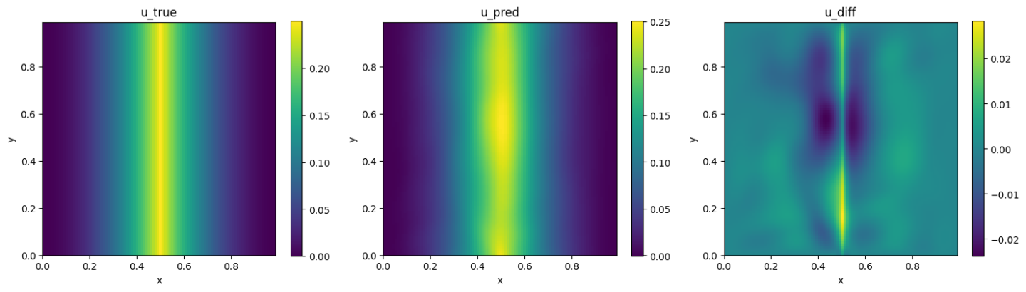
Fig. 105 Left: PhysicsNeMo Sym. Center: Analytical. Right: Difference.
By using quadrature rule, the results are shown in Fig. 106.

Fig. 106 Left: PhysicsNeMo Sym. Center: Analytical. Right: Difference.
By using quadrature rule and RBF test function, the results are shown in Fig. 107.

Fig. 107 Left: PhysicsNeMo Sym. Center: Analytical. Right: Difference.
Weak formulation enables solution of PDEs with distributions, e.g., Dirac Delta function. The Dirac Delta function \(\delta(x)\) is defined as
(185)\[\int_{\mathbb{R}}f(x)\delta(x) dx = f(0),\]
for all continuous compactly supported functions \(f\).
This subsection solves the following problem:
(186)\[\begin{split}\begin{aligned}
-\Delta u &= \delta \quad \mbox{ in } \Omega\\
u &= 0 \quad \text{ on } \partial\Omega\end{aligned}\end{split}\]
where \(\Omega=(-0.5,0.5)^2\) (Fig. 108). In physics, this means there is a point source in the middle of the domain with \(0\) Lebesgue measure in \(\mathbb{R}^2\). The corresponding weak formulation is
(187)\[\int_{\Omega}\nabla u\cdot \nabla v dx - \int_{\Gamma} \frac{\partial u}{\partial \mathbf{n}}v ds = v(0, 0)\]
The code of this example can be found in ./point_source/point_source.py.

Fig. 108 Domain for the point source problem.
Creating the Geometry
Use both the weak and differential form to solve (186) and (187). Since the solution has a sharp gradient around the origin, which causes issues for traditional PINNs, weight this area lower using the lambda weighting functions. The geometry can be defined by:
            x, y = Symbol("x"), Symbol("y")

    # make geometry
Creating the Variational Loss and Solver
As shown in (187), the only difference to the
previous examples is the right hand side term is the value of \(v\)
instead of an integral. You only need to change the fv in the
code. The whole code of the DGLoss is the following:
            rec = Rectangle((-0.5, -0.5), (0.5, 0.5))

    # make domain
    domain = Domain()

    Wall = PointwiseBoundaryConstraint(
        nodes=nodes,
        geometry=rec,
        outvar={"u": 0.0},
        lambda_weighting={"u": 10.0},
        batch_size=cfg.batch_size.boundary,
        fixed_dataset=False,
        batch_per_epoch=1,
        quasirandom=True,
    )
    domain.add_constraint(Wall, name="OutsideWall")

    # PINN constraint
    interior = PointwiseInteriorConstraint(
        nodes=nodes,
        geometry=rec,
        outvar={"diffusion_u": 0.0},
        batch_size=cfg.batch_size.interior,
        bounds=Bounds({x: (-0.5, 0.5), y: (-0.5, 0.5)}),
        lambda_weighting={"diffusion_u": (x**2 + y**2)},
        fixed_dataset=False,
        batch_per_epoch=1,
        quasirandom=True,
    )
    domain.add_constraint(interior, "interior")

    # Variational contraint
    variational = VariationalDomainConstraint(
        nodes=nodes,
        geometry=rec,
        outvar_names=["u__x", "u__y"],
        boundary_batch_size=cfg.batch_size.boundary,
        interior_batch_size=cfg.batch_size.interior,
        interior_bounds=Bounds({x: (-0.5, 0.5), y: (-0.5, 0.5)}),
        loss=DGLoss(),
        batch_per_epoch=1,
        quasirandom=True,
    )
    domain.add_constraint(variational, "variational")

    # add inferencer data
    inferencer = PointwiseInferencer(
        nodes=nodes,
        invar=rec.sample_interior(10000),
        output_names=["u"],
        batch_size=2048,
        plotter=InferencerPlotter(),
    )
    domain.add_inferencer(inferencer)

    # make solver
    slv = Solver(cfg, domain)
Results and Post-processing
The results for the problem are shown in Fig. 109.

Fig. 109 PhysicsNeMo Sym prediction
Since the ground truth solution is unbounded at origin, it is not useful to compare it with the exact solution.