Triton Architecture
Contents
Triton Architecture#
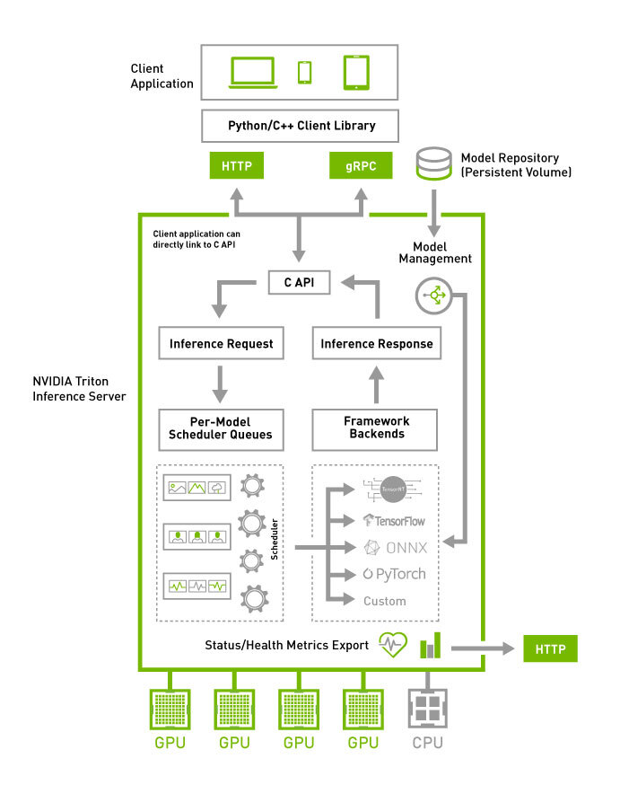
The following figure shows the Triton Inference Server high-level architecture. The model repository is a file-system based repository of the models that Triton will make available for inferencing. Inference requests arrive at the server via either HTTP/REST or GRPC or by the C API and are then routed to the appropriate per-model scheduler. Triton implements multiple scheduling and batching algorithms that can be configured on a model-by-model basis. Each model’s scheduler optionally performs batching of inference requests and then passes the requests to the backend corresponding to the model type. The backend performs inferencing using the inputs provided in the batched requests to produce the requested outputs. The outputs are then returned.
Triton supports a backend C API that allows Triton to be extended with new functionality such as custom pre- and post-processing operations or even a new deep-learning framework.
The models being served by Triton can be queried and controlled by a dedicated model management API that is available by HTTP/REST or GRPC protocol, or by the C API.
Readiness and liveness health endpoints and utilization, throughput and latency metrics ease the integration of Triton into deployment framework such as Kubernetes.
Concurrent Model Execution#
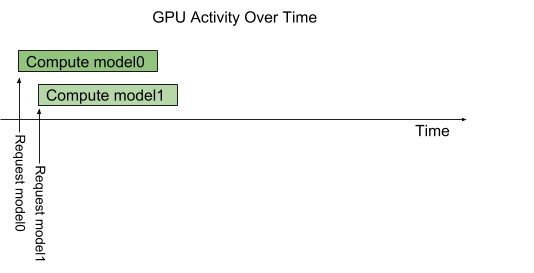
The Triton architecture allows multiple models and/or multiple instances of the same model to execute in parallel on the same system. The system may have zero, one, or many GPUs. The following figure shows an example with two models; model0 and model1. Assuming Triton is not currently processing any request, when two requests arrive simultaneously, one for each model, Triton immediately schedules both of them onto the GPU and the GPU’s hardware scheduler begins working on both computations in parallel. Models executing on the system’s CPU are handled similarly by Triton except that the scheduling of the CPU threads execution each model is handled by the system’s OS.
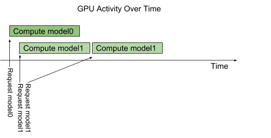
By default, if multiple requests for the same model arrive at the same time, Triton will serialize their execution by scheduling only one at a time on the GPU, as shown in the following figure.
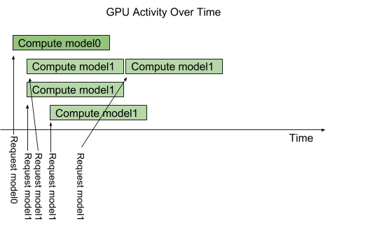
Triton provides a model configuration option called instance-group that allows each model to specify how many parallel executions of that model should be allowed. Each such enabled parallel execution is referred to as an instance. By default, Triton gives each model a single instance for each available GPU in the system. By using the instance_group field in the model configuration, the number of execution instances for a model can be changed. The following figure shows model execution when model1 is configured to allow three instances. As shown in the figure, the first three model1 inference requests are immediately executed in parallel. The fourth model1 inference request must wait until one of the first three executions completes before beginning.
Models And Schedulers#
Triton supports multiple scheduling and batching algorithms that can be selected independently for each model. This section describes stateless, stateful and ensemble models and how Triton provides schedulers to support those model types. For a given model, the selection and configuration of the scheduler is done with the model’s configuration file.
Stateless Models#
With respect to Triton’s schedulers, a stateless model does not maintain state between inference requests. Each inference performed on a stateless model is independent of all other inferences using that model.
Examples of stateless models are CNNs such as image classification and object detection. The default scheduler or dynamic batcher can be used as the scheduler for these stateless models.
RNNs and similar models which do have internal memory can be stateless as long as the state they maintain does not span inference requests. For example, an RNN that iterates over all elements in a batch is considered stateless by Triton if the internal state is not carried between batches of inference requests. The default scheduler can be used for these stateless models. The dynamic batcher cannot be used since the model is typically not expecting the batch to represent multiple inference requests.
Stateful Models#
With respect to Triton’s schedulers, a stateful model does maintain state between inference requests. The model is expecting multiple inference requests that together form a sequence of inferences that must be routed to the same model instance so that the state being maintained by the model is correctly updated. Moreover, the model may require that Triton provide control signals indicating, for example, the start and end of the sequence.
The sequence batcher must be used for these stateful models. As explained below, the sequence batcher ensures that all inference requests in a sequence get routed to the same model instance so that the model can maintain state correctly. The sequence batcher also communicates with the model to indicate when a sequence is starting, when a sequence is ending, when a sequence has an inference request ready for execution, and the correlation ID of the sequence.
When making inference requests for a stateful model, the client application must provide the same correlation ID to all requests in a sequence, and must also mark the start and end of the sequence. The correlation ID allows Triton to identify that the requests belong to the same sequence.
Control Inputs#
For a stateful model to operate correctly with the sequence batcher, the model must typically accept one or more control input tensors that Triton uses to communicate with the model. The ModelSequenceBatching::Control section of the model configuration indicates how the model exposes the tensors that the sequence batcher should use for these controls. All controls are optional. Below is portion of a model configuration that shows an example configuration for all the available control signals.
sequence_batching {
  control_input [
    {
      name: "START"
      control [
        {
          kind: CONTROL_SEQUENCE_START
          fp32_false_true: [ 0, 1 ]
        }
      ]
    },
    {
      name: "END"
      control [
        {
          kind: CONTROL_SEQUENCE_END
          fp32_false_true: [ 0, 1 ]
        }
      ]
    },
    {
      name: "READY"
      control [
        {
          kind: CONTROL_SEQUENCE_READY
          fp32_false_true: [ 0, 1 ]
        }
      ]
    },
    {
      name: "CORRID"
      control [
        {
          kind: CONTROL_SEQUENCE_CORRID
          data_type: TYPE_UINT64
        }
      ]
    }
  ]
}
Start: The start input tensor is specified using CONTROL_SEQUENCE_START in the configuration. The example configuration indicates that the model has an input tensor called START with a 32-bit floating point data-type. The sequence batcher will define this tensor when executing an inference on the model. The START tensor must be 1-dimensional with size equal to the batch-size. Each element in the tensor indicates if the sequence in the corresponding batch slot is starting or not. In the example configuration, fp32_false_true indicates that a sequence start is indicated by tensor element equal to 1, and non-start is indicated by tensor element equal to 0.
End: The end input tensor is specified using CONTROL_SEQUENCE_END in the configuration. The example configuration indicates that the model has an input tensor called END with a 32-bit floating point data-type. The sequence batcher will define this tensor when executing an inference on the model. The END tensor must be 1-dimensional with size equal to the batch-size. Each element in the tensor indicates if the sequence in the corresponding batch slot is ending or not. In the example configuration, fp32_false_true indicates that a sequence end is indicated by tensor element equal to 1, and non-end is indicated by tensor element equal to 0.
Ready: The ready input tensor is specified using CONTROL_SEQUENCE_READY in the configuration. The example configuration indicates that the model has an input tensor called READY with a 32-bit floating point data-type. The sequence batcher will define this tensor when executing an inference on the model. The READY tensor must be 1-dimensional with size equal to the batch-size. Each element in the tensor indicates if the sequence in the corresponding batch slot has an inference request ready for inference. In the example configuration, fp32_false_true indicates that a sequence ready is indicated by tensor element equal to 1, and non-ready is indicated by tensor element equal to 0.
Correlation ID: The correlation ID input tensor is specified using CONTROL_SEQUENCE_CORRID in the configuration. The example configuration indicates that the model has an input tensor called CORRID with a unsigned 64-bit integer data-type. The sequence batcher will define this tensor when executing an inference on the model. The CORRID tensor must be 1-dimensional with size equal to the batch-size. Each element in the tensor indicates the correlation ID of the sequence in the corresponding batch slot.
Implicit State Management#
Implicit state management allows a stateful model to store its state inside Triton. When using implicit state, the stateful model does not need to store the state required for inference inside the model.
Below is a portion of the model configuration that indicates the model is using implicit state.
sequence_batching {
  state [
    {
      input_name: "INPUT_STATE"
      output_name: "OUTPUT_STATE"
      data_type: TYPE_INT32
      dims: [ -1 ]
    }
  ]
}
The state section in the sequence_batching setting is used to indicate that the model is using implicit state. The input_name field specifies the name of the input tensor that will contain the input state. The output_name field describes the name of the output tensor produced by the model that contains output state. The output state provided by the model in the ith request in the sequence will be used as the input state in the i+1th request. The dims field specifies the dimensions of the state tensors. When the dims field contains variable-sized dimensions, the shape of the input state and output state does not have to match.
For debugging purposes, the client can request the output state. In order to allow the client to request the output state, the output section of the model configuration must list the output state as one of the model outputs. Note that requesting the output state from the client can increase the request latency because of the additional tensors that have to be transferred.
Implicit state management requires backend support. Currently, only onnxruntime_backend and tensorrt_backend support implicit state.
State Initialization#
By default, the starting request in the sequence contains uninitialized data for
the input state. The model can use the start flag in the request to detect the
beginning of a new sequence and initialize the model state by providing the
initial state in the model output. If the dims section in the state
description of the model contains variable-sized dimensions, Triton will use 1
for every variable-sized dimension for the starting request. For other
non-starting requests in the sequence, the input state is the output state of
the previous request in the sequence. For an example ONNX model that uses
implicit state you can refer to this onnx model generated from the
create_onnx_modelfile_wo_initial_state()
from this generation script.
This is a simple accumulator model that stores the partial sum of the requests
in a sequence in Triton using implicit state. For state initialization, if the
request is starting, the model sets the “OUTPUT_STATE” to be equal to the
“INPUT” tensor. For non-starting requests, it sets the “OUTPUT_STATE” tensor
to the sum of “INPUT” and “INPUT_STATE” tensors.
In addition to the default state initilization discussed above, Triton provides two other mechanisms for initilizing state.
Initializing State from Zero.#
Below is an example of initializing state from zero.
sequence_batching {
  state [
    {
      input_name: "INPUT_STATE"
      output_name: "OUTPUT_STATE"
      data_type: TYPE_INT32
      dims: [ -1 ]
      initial_state: {
       data_type: TYPE_INT32
       dims: [ 1 ]
       zero_data: true
       name: "initial state"
      }
    }
  ]
}
Note that in the example above variable dimensions in the state description are converted to fixed size dimensions.
Initializing State from File#
For initializing state from file, you need to create a directory named “initial_state” under the model directory. The file that contains the initial state under this directory needs to be provided in the data_file field. The data stored in this file will be used in row-major order as the initial state. Below is an example state description initializing state from file.
sequence_batching {
  state [
    {
      input_name: "INPUT_STATE"
      output_name: "OUTPUT_STATE"
      data_type: TYPE_INT32
      dims: [ -1 ]
      initial_state: {
       data_type: TYPE_INT32
       dims: [ 1 ]
       data_file: "initial_state_data"
       name: "initial state"
      }
    }
  ]
}
Scheduling Strategies#
The sequence batcher can employ one of two scheduling strategies when deciding how to batch the sequences that are routed to the same model instance. These strategies are direct and oldest.
Direct#
With the Direct scheduling strategy the sequence batcher ensures not only that all inference requests in a sequence are routed to the same model instance, but also that each sequence is routed to a dedicated batch slot within the model instance. This strategy is required when the model maintains state for each batch slot, and is expecting all inference requests for a given sequence to be routed to the same slot so that the state is correctly updated.
As an example of the sequence batcher using the Direct scheduling strategy, assume a TensorRT stateful model that has the following model configuration.
name: "direct_stateful_model"
platform: "tensorrt_plan"
max_batch_size: 2
sequence_batching {
  max_sequence_idle_microseconds: 5000000
  direct { }
  control_input [
    {
      name: "START"
      control [
        {
          kind: CONTROL_SEQUENCE_START
          fp32_false_true: [ 0, 1 ]
        }
      ]
    },
    {
      name: "READY"
      control [
        {
          kind: CONTROL_SEQUENCE_READY
          fp32_false_true: [ 0, 1 ]
        }
      ]
    }
  ]
}
input [
  {
    name: "INPUT"
    data_type: TYPE_FP32
    dims: [ 100, 100 ]
  }
]
output [
  {
    name: "OUTPUT"
    data_type: TYPE_FP32
    dims: [ 10 ]
  }
]
instance_group [
  {
    count: 2
  }
]
The sequence_batching section indicates that the model should use the sequence batcher and the Direct scheduling strategy. In this example the model only requires a start and ready control input from the sequence batcher so only those controls are listed. The instance_group indicates two instances of the model should be instantiated and max_batch_size indicates that each of those instances should perform batch-size 2 inferences. The following figure shows a representation of the sequence batcher and the inference resources specified by this configuration.
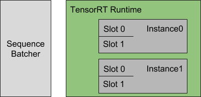
Each model instance is maintaining state for each batch slot, and is expecting all inference requests for a given sequence to be routed to the same slot so that the state is correctly updated. For this example that means that Triton can simultaneously perform inference for up to four sequences.
Using the Direct scheduling strategy, the sequence batcher:
Recognizes when an inference request starts a new sequence and allocates a batch slot for that sequence. If no batch slot is available for the new sequence, Triton places the inference request in a backlog.
Recognizes when an inference request is part of a sequence that has an allocated batch slot and routes the request to that slot.
Recognizes when an inference request is part of a sequence that is in the backlog and places the request in the backlog.
Recognizes when the last inference request in a sequence has been completed. The batch slot occupied by that sequence is immediately reallocated to a sequence in the backlog, or freed for a future sequence if there is no backlog.
The following figure shows how multiple sequences are scheduled onto the model instances using the Direct scheduling strategy. On the left the figure shows several sequences of requests arriving at Triton. Each sequence could be made up of any number of inference requests and those individual inference requests could arrive in any order relative to inference requests in other sequences, except that the execution order shown on the right assumes that the first inference request of sequence 0 arrives before any inference request in sequences 1-5, the first inference request of sequence 1 arrives before any inference request in sequences 2-5, etc.
The right of the figure shows how the inference request sequences are scheduled onto the model instances over time.

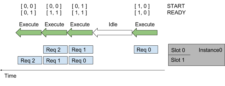
The following figure shows the sequence batcher uses the control input tensors to communicate with the model. The figure shows two sequences assigned to the two batch slots in a model instance. Inference requests for each sequence arrive over time. The START and READY rows show the input tensor values used for each execution of the model. Over time the following happens:
The first request arrives for the sequence in slot0. Assuming the model instance is not already executing an inference, the sequence scheduler immediately schedules the model instance to execute because an inference request is available.
This is the first request in the sequence so the corresponding element in the START tensor is set to 1. There is no request available in slot1 so the READY tensor shows only slot0 as ready.
After the inference completes the sequence scheduler sees that there are no requests available in any batch slot and so the model instance sits idle.
Next, two inference requests arrive close together in time so that the sequence scheduler sees them both available in their respective batch slots. The scheduler immediately schedules the model instance to perform a batch-size 2 inference and uses START and READY to show that both slots have an inference request avaiable but that only slot1 is the start of a new sequence.
The processing continues in a similar manner for the other inference requests.
Oldest#
With the Oldest scheduling strategy the sequence batcher ensures that all inference requests in a sequence are routed to the same model instance and then uses the dynamic batcher to batch together multiple inferences from different sequences into a batch that inferences together. With this strategy the model must typically use the CONTROL_SEQUENCE_CORRID control so that it knows which sequence each inference request in the batch belongs to. The CONTROL_SEQUENCE_READY control is typically not needed because all inferences in the batch will always be ready for inference.
As an example of the sequence batcher using the Oldest scheduling strategy, assume a stateful model that has the following model configuration:
name: "oldest_stateful_model"
platform: "tensorflow_savedmodel"
max_batch_size: 2
sequence_batching {
  max_sequence_idle_microseconds: 5000000
  oldest
    {
      max_candidate_sequences: 4
    }
  control_input [
    {
      name: "START"
      control [
        {
          kind: CONTROL_SEQUENCE_START
          fp32_false_true: [ 0, 1 ]
        }
      ]
    },
    {
      name: "END"
      control [
        {
          kind: CONTROL_SEQUENCE_END
          fp32_false_true: [ 0, 1 ]
        }
      ]
    },
    {
      name: "CORRID"
      control [
        {
          kind: CONTROL_SEQUENCE_CORRID
          data_type: TYPE_UINT64
        }
      ]
    }
  ]
}
input [
  {
    name: "INPUT"
    data_type: TYPE_FP32
    dims: [ 100, 100 ]
  }
]
output [
  {
    name: "OUTPUT"
    data_type: TYPE_FP32
    dims: [ 10 ]
  }
]
The sequence_batching section indicates that the model should use the sequence batcher and the Oldest scheduling strategy. The Oldest strategy is configured so that the sequence batcher maintains up to 4 active candidate sequences from which it prefers to form dynamic batches of size 2. In this example the model requires a start, end, and correlation ID control input from the sequence batcher. The following figure shows a representation of the sequence batcher and the inference resources specified by this configuration.
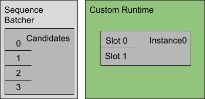
Using the Oldest scheduling strategy, the sequence batcher:
Recognizes when an inference request starts a new sequence and attempts to find a model instance that has room for a candidate sequence. If no model instance has room for a new candidate sequence, Triton places the inference request in a backlog.
Recognizes when an inference request is part of a sequence that is already a candidate sequence in some model instance and routes the request to that model instance.
Recognizes when an inference request is part of a sequence that is in the backlog and places the request in the backlog.
Recognizes when the last inference request in a sequence has been completed. The model instance immediately removes a sequence from the backlog and makes it a candidate sequence in the model instance, or records that the model instance can handle a future sequence if there is no backlog.
The following figure shows how multiple sequences are scheduled onto the model instance specified by the above example configuration. On the left the figure shows four sequences of requests arriving at Triton. Each sequence is composed of multiple inference requests as shown in the figure. The center of the figure shows how the inference request sequences are batched onto the model instance over time, assuming that the inference requests for each sequence arrive at the same rate with sequence A arriving just before B, which arrives just before C, etc. The Oldest strategy forms a dynamic batch from the oldest requests but never includes more than one request from a given sequence in a batch (for example, the last two inferences in sequence D are not batched together).

Ensemble Models#
An ensemble model represents a pipeline of one or more models and the connection of input and output tensors between those models. Ensemble models are intended to be used to encapsulate a procedure that involves multiple models, such as “data preprocessing -> inference -> data postprocessing”. Using ensemble models for this purpose can avoid the overhead of transferring intermediate tensors and minimize the number of requests that must be sent to Triton.
The ensemble scheduler must be used for ensemble models, regardless of the scheduler used by the models within the ensemble. With respect to the ensemble scheduler, an ensemble model is not an actual model. Instead, it specifies the dataflow between models within the ensemble as ModelEnsembling::Step entries in the model configuration. The scheduler collects the output tensors in each step, provides them as input tensors for other steps according to the specification. In spite of that, the ensemble model is still viewed as a single model from an external view.
Note that the ensemble models will inherit the characteristics of the models involved, so the meta-data in the request header must comply with the models within the ensemble. For instance, if one of the models is stateful model, then the inference request for the ensemble model should contain the information mentioned in Stateful Models, which will be provided to the stateful model by the scheduler.
As an example consider an ensemble model for image classification and segmentation that has the following model configuration:
name: "ensemble_model"
platform: "ensemble"
max_batch_size: 1
input [
  {
    name: "IMAGE"
    data_type: TYPE_STRING
    dims: [ 1 ]
  }
]
output [
  {
    name: "CLASSIFICATION"
    data_type: TYPE_FP32
    dims: [ 1000 ]
  },
  {
    name: "SEGMENTATION"
    data_type: TYPE_FP32
    dims: [ 3, 224, 224 ]
  }
]
ensemble_scheduling {
  step [
    {
      model_name: "image_preprocess_model"
      model_version: -1
      input_map {
        key: "RAW_IMAGE"
        value: "IMAGE"
      }
      output_map {
        key: "PREPROCESSED_OUTPUT"
        value: "preprocessed_image"
      }
    },
    {
      model_name: "classification_model"
      model_version: -1
      input_map {
        key: "FORMATTED_IMAGE"
        value: "preprocessed_image"
      }
      output_map {
        key: "CLASSIFICATION_OUTPUT"
        value: "CLASSIFICATION"
      }
    },
    {
      model_name: "segmentation_model"
      model_version: -1
      input_map {
        key: "FORMATTED_IMAGE"
        value: "preprocessed_image"
      }
      output_map {
        key: "SEGMENTATION_OUTPUT"
        value: "SEGMENTATION"
      }
    }
  ]
}
The ensemble_scheduling section indicates that the ensemble scheduler will be used and that the ensemble model consists of three different models. Each element in step section specifies the model to be used and how the inputs and outputs of the model are mapped to tensor names recognized by the scheduler. For example, the first element in step specifies that the latest version of image_preprocess_model should be used, the content of its input “RAW_IMAGE” is provided by “IMAGE” tensor, and the content of its output “PREPROCESSED_OUTPUT” will be mapped to “preprocessed_image” tensor for later use. The tensor names recognized by the scheduler are the ensemble inputs, the ensemble outputs and all values in the input_map and the output_map.
The models composing the ensemble may also have dynamic batching enabled. Since ensemble models are just routing the data between composing models, Triton can take requests into an ensemble model without modifying the ensemble’s configuration to exploit the dynamic batching of the composing models.
Assuming that only the ensemble model, the preprocess model, the classification model and the segmentation model are being served, the client applications will see them as four different models which can process requests independently. However, the ensemble scheduler will view the ensemble model as the following.
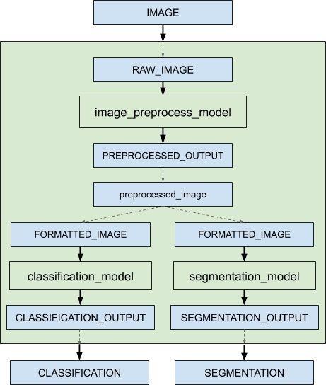
When an inference request for the ensemble model is received, the ensemble scheduler will:
Recognize that the “IMAGE” tensor in the request is mapped to input “RAW_IMAGE” in the preprocess model.
Check models within the ensemble and send an internal request to the preprocess model because all the input tensors required are ready.
Recognize the completion of the internal request, collect the output tensor and map the content to “preprocessed_image” which is an unique name known within the ensemble.
Map the newly collected tensor to inputs of the models within the ensemble. In this case, the inputs of “classification_model” and “segmentation_model” will be mapped and marked as ready.
Check models that require the newly collected tensor and send internal requests to models whose inputs are ready, the classification model and the segmentation model in this case. Note that the responses will be in arbitrary order depending on the load and computation time of individual models.
Repeat step 3-5 until no more internal requests should be sent, and then response to the inference request with the tensors mapped to the ensemble output names.
Additional Resources#
You can find additional end-to-end ensemble examples in the links below:
