

GPU Sharing
GPU sharing enables many lightly-used models to run on the same GPU. Dynamo offers multiple paths - MIG, MPS, HAMi and GPU fractions, offering various levels of isolation - to enable sharing a GPU. This page compares serving one model per GPU against packing two models onto a GPU and walks you through evaluating the throughput and latency tradeoffs involved.
Setup
We ran the same models on an 8× A100 node with Qwen3-4B, with a fixed input length of 2048 tokens, and a fixed output length of 256 tokens.
The results are pessimistic: they assume no KV caching between requests, so the entire 2048-token input sequence length (ISL) is computed on every request.
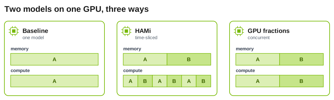
In the HAMi and GPU fractions configurations, each model receives half of the GPU memory. With GPU fractions, each model’s MPS compute limit is also set to half of the GPU’s streaming multiprocessors (SMs).
- Time-slicing: both models share all of the GPU’s SMs, and the CUDA driver context switches between them, so one model’s work waits while the other’s runs.
- GPU fractioning: each model gets a memory cap and an MPS limit on the share of SMs it can use, so both models can run concurrently instead of taking turns. The limit caps a model’s share. It does not reserve specific SMs.
The configurations are built from these components:
- KAI-Scheduler: an open-source Kubernetes scheduler that can place a pod on a fraction of a GPU. A pod asks for a share with
gpu-fraction: "0.5". Both shared configurations use it. The baseline requests whole GPUs. - HAMi: a resource isolator that enforces a per-pod GPU memory cap. It does not partition compute, so the CUDA driver time-slices the models on a GPU.
- MPS: the CUDA Multi-Process Service lets processes share a GPU at the same time and caps the share of SMs each client can use. MPS v3 namespaces give each pod its own limits.
- GPU fractions: KAI-Scheduler and kai-gpu-fractioning, built from forks, with each pod running in its own MPS namespace. The scheduler tracks compute as well as memory, MPS enforces the SM share limit, and the driver enforces the memory cap.
GPU Sharing Benchmark Results (Experimental)
These results are experimental. More extensive benchmarks are coming soon. Any performance results on this page are purely illustrative and are not indicative of optimal performance. Your deployment or configuration may vary.
Throughput
Concurrency, c, is defined as the number of concurrent requests each model has in flight. A shared GPU hosts two models, so HAMi and GPU fractions at c=1 place the same two requests on each GPU as vanilla at c=2. The first column, Requests resident/GPU, is that shared quantity. Each row compares the three configurations under the same pressure on the hardware.
Note that we expect degradation in the model performance since we are sharing the compute of the gpu between two distinct models. We highlight that using the fractional gpu method, limiting each model’s share of the SMs and HBM memory, we get better performance packing multiple models onto one gpu than when using the previous state of the art, KAI+HAMi, only partitioning the memory and time-slicing the compute.
TTFT p50 (ms)
ITL p50 (ms)
Cost per 1M Output Tokens
This table compares the cost of serving 16 models when each model receives the same traffic. Serving 16 models with one model per GPU requires leasing two 8× A100 nodes, while GPU fractions serves all 16 on one node. The baseline is extrapolated from the 8-model run by doubling its throughput. Both configurations are priced at a normalized /1M columns by your node-hour price to get your cost. The percentage column does not depend on the price.
Unlike the tables above, rows here are matched on concurrency per model, not requests per GPU.
$/1M is the hourly node cost divided by output tokens per hour, scaled to one million tokens. Only output tokens are counted. At light per-model load, a dedicated GPU sits mostly idle, and packing two models onto it recovers that idle capacity. At 32 concurrent requests per model, the dedicated GPUs are busy enough that the cost advantage disappears.
How to Read the Benchmark
Read across a row to confirm that latency meets your requirements, then use Fractions % of Baseline to decide whether giving up that share of throughput is worth one GPU saved per pair of models.
Rows are matched on load per GPU
Each row compares the configurations at the same number of requests resident on each GPU. A shared GPU hosts two models, so HAMi and GPU fractions at concurrency c match the baseline at concurrency 2c.
Comparing rows at equal c instead would give the shared configurations twice the load of the baseline and make them look better than they are.
Latency columns
TTFT p50 (time to first token) and ITL p50 (inter-token latency) are per-request medians. Sharing always costs latency, because each model runs on only part of the GPU. Treat these columns as a check that latency is still acceptable for your service. GPU fractions matches or beats HAMi on ITL in every row, and ITL stays under 30 ms throughout.
Throughput columns
tok/s per GPU is output tokens per second per GPU, summed across all models on that GPU. The absolute values depend on this model, GPU, and prompt shape, so they do not carry over to your workload.
Percentage columns
Fractions % of Baseline answers the deployment question directly: when you put two models on one GPU instead of giving each its own, how much of that GPU’s throughput do you keep?
Base decisions on the percentage columns for three reasons:
- They cancel out the setup. Model size, GPU type, and sequence lengths shift all three configurations together. A ratio against a dedicated baseline at the same load isolates the cost of sharing, which makes it the number most likely to transfer to your workload.
- They map to a GPU-count decision. At one request per model, GPU fractions keeps 63.5%: one GPU serves two distinct models at about 63% of the throughput a dedicated GPU would deliver, rising to 87.9% at 16 requests per model. For every pair of models that can tolerate that, you free a whole GPU. In this benchmark, 16 models run on 8 GPUs instead of 16.
- They separate how the GPU is shared from the fact that it is shared. HAMi and GPU fractions both pay the cost of splitting a GPU. The 15 to 20 point gap between them is the gain from limiting each model’s share of compute with MPS instead of time-slicing it. Under time-slicing, one model’s kernels wait behind the other’s. With MPS limits, both models’ kernels can run at the same time. The limit caps a model’s share of SMs but does not guarantee that its kernels start immediately when its neighbor is busy.
Why sharing costs throughput
Each decode step reads the model’s full weights from GPU memory, and at low load that read dominates the step time. One model serving two requests reads its weights once per step for both. Two models serving one request each read two sets of weights, which roughly doubles the memory traffic for the same output. At low load this duplication dominates, and GPU fractions keeps about 63% of dedicated throughput.
As load rises, each step does more compute per weight read, so the duplicated reads matter less. GPU fractions climbs to about 88% of dedicated throughput at 32 requests per GPU.
Reproducing the Results
The manifests, scripts, and step-by-step guides for every configuration are in the examples/gpu-sharing directory on GitHub. Start with its README, which covers the shared workload, the files, and the commands.
Appendix: Node Throughput at Equal Per-Model Concurrency
This table compares total node output throughput (tok/s) with every configuration at the same per-model concurrency. The shared configurations run 16 models on 8 GPUs, so each GPU carries twice as many in-flight requests as in the vanilla configuration at the same c/model.