Core Concepts and Your First Simulation

In this lesson, we’ll meet the handful of abstractions that every Newton simulation is built from, assemble a minimal scene, and step it forward in time. We’ll finish by accelerating the loop with CUDA graph capture and measuring the speedup for ourselves.

Tip

Short on time? Jump to the final example for the complete runnable script.

In this lesson, we will:

• Describe the roles of ModelBuilder, Model, State, Control, Contacts, and Solver.

• Build a two-object scene and finalize it into a simulation-ready Model.

• Step the simulation with a solver and watch it live in the viewer.

• Apply CUDA graph capture and compare timings.

Setup and Imports

We use Warp for numerical compute and Newton for simulation. Setting wp.config.quiet = True keeps Warp’s logging tidy while kernels compile.

import numpy as np
import warp as wp

import newton
import newton.examples
import newton.utils
import newton.ik as ik

wp.config.quiet = True

newton.solvers.SolverMuJoCo.import_mujoco()

We’ll also reuse one small helper throughout the module. The make_viewer() function opens a Viser web viewer. Before running a script, open http://localhost:8080 in a browser tab. Reload that tab when the Viser server starts so the simulation does not finish before you open the viewer.

from pathlib import Path


def make_viewer(name: str):
    """Open a Viser web viewer; it prints a URL (normally http://localhost:8080)."""
    return newton.viewer.ViewerViser(verbose=False)

Note

The interactive notebook version of this module also defines HTML progress-bar and diagram helpers for display inside Jupyter. Those are cosmetic and notebook-only, so the run-at-home scripts below use plain loops instead.

The Newton Building Blocks

Newton simulations revolve around a small set of core abstractions:

• ModelBuilder is the construction API. You use it to import assets from USD, MJCF, or URDF and to assemble bodies, shapes, joints, and their properties.

• Model is the compiled, simulation-ready data (arrays and metadata) that lives on the compute device.

• State holds time-varying data such as positions, velocities, and forces.

• Control holds the control inputs for joints, such as target positions and torques.

• Contacts holds the geometric contact information produced by the collision-detection pipeline.

• Solver advances the simulation by integrating physics and resolving constraints.

In each substep, the solver consumes the model, state, control, and contacts plus a timestep dt, and writes the next state. Everything else in this module is a variation on that single idea.

Newton Is Built on NVIDIA Warp

Warp is NVIDIA’s Python framework for writing high-performance simulation and geometry code without hand-writing CUDA. You write kernels in Python (for example with @wp.kernel), and Warp just-in-time compiles them into optimized native code that runs on the CPU or GPU. In practice, Warp gives you a Python workflow with near low-level performance for physics, robotics, and graphics workloads. The first time you launch a kernel, Warp parses it, generates CUDA C++, and compiles it, so the first step of any simulation is always the slowest.

Building a Scene: ModelBuilder to Model

Let’s build a minimal scene: a ground plane, one box, and one sphere. Keeping the scene small lets us focus on the API.

builder = newton.ModelBuilder()

# Static ground
builder.add_ground_plane()

# Dynamic box
box_body = builder.add_body(xform=wp.transform(wp.vec3(0.0, -1.0, 1.0), wp.quat_identity()))
builder.add_shape_box(box_body, hx=0.15, hy=0.15, hz=0.15)

# Dynamic sphere
sphere_body = builder.add_body(xform=wp.transform(wp.vec3(0.0, 1.0, 1.2), wp.quat_identity()))
builder.add_shape_sphere(sphere_body, radius=0.18)

print(f"Bodies: {builder.body_count}, Shapes: {builder.shape_count}")

Each add_body call registers a rigid body at a world transform, and each add_shape_* call attaches collision and visual geometry to a body.

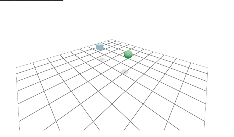
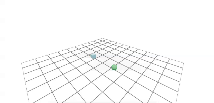
The assembled scene rendered in the Viser viewer: a ground plane, one box, and one sphere before stepping the solver.

Finalize Into a Model, State, Control, and Contacts

Finalizing converts the builder into a device-ready Model. From that model we allocate two State objects, one Control, and one reusable Contacts buffer. We use two states so the solver can read from one and write into the other, then swap them.

model = builder.finalize()

state_0 = model.state()
state_1 = model.state()
control = model.control()
collision_pipeline = newton.CollisionPipeline(model)
contacts = collision_pipeline.contacts()

print(f"Model device: {model.device}")
print(f"Body count: {model.body_count}")

Contacts is populated by the collision pipeline at each substep and passed into solver.step(...) alongside state, control, and dt.

Tip

In the Viser viewer you can orbit the camera by dragging with the left mouse button, pan by dragging with the right mouse button, and zoom with the mouse wheel.

The Solver and Simulation Loop

We’ll use the XPBD solver for this tiny scene. The loop always follows the same pattern: clear forces, collide, step, then swap the state buffers.

solver = newton.solvers.SolverXPBD(model, iterations=10)

fps = 60
frame_dt = 1.0 / fps
sim_substeps = 8
sim_dt = frame_dt / sim_substeps


def simulate():
    global state_0, state_1

    for _ in range(sim_substeps):
        state_0.clear_forces()
        collision_pipeline.collide(state_0, contacts)
        solver.step(state_in=state_0, state_out=state_1, control=control, contacts=contacts, dt=sim_dt)
        state_0, state_1 = state_1, state_0

We run several substeps per rendered frame. Smaller substeps improve stability at the cost of compute.

Visualize the Simulation

We open a ViewerViser window and log each frame as simulate() advances the scene. Reload the http://localhost:8080 browser tab you opened before starting the script to watch it live.

viewer = make_viewer("01_simple_scene")
viewer.set_model(model)

print("Starting simulation, this may take a minute to compile the CUDA kernels...")

sim_time = 0.0
num_frames = 180
for _ in range(num_frames):
    simulate()
    viewer.begin_frame(sim_time)
    viewer.log_state(state_0)
    viewer.end_frame()
    sim_time += frame_dt

Watch the box and sphere fall under gravity and settle on the ground plane.

In the viewer: the box and sphere drop from their initial poses, bounce slightly, and come to rest on the ground.

Accelerating With CUDA Graph Capture

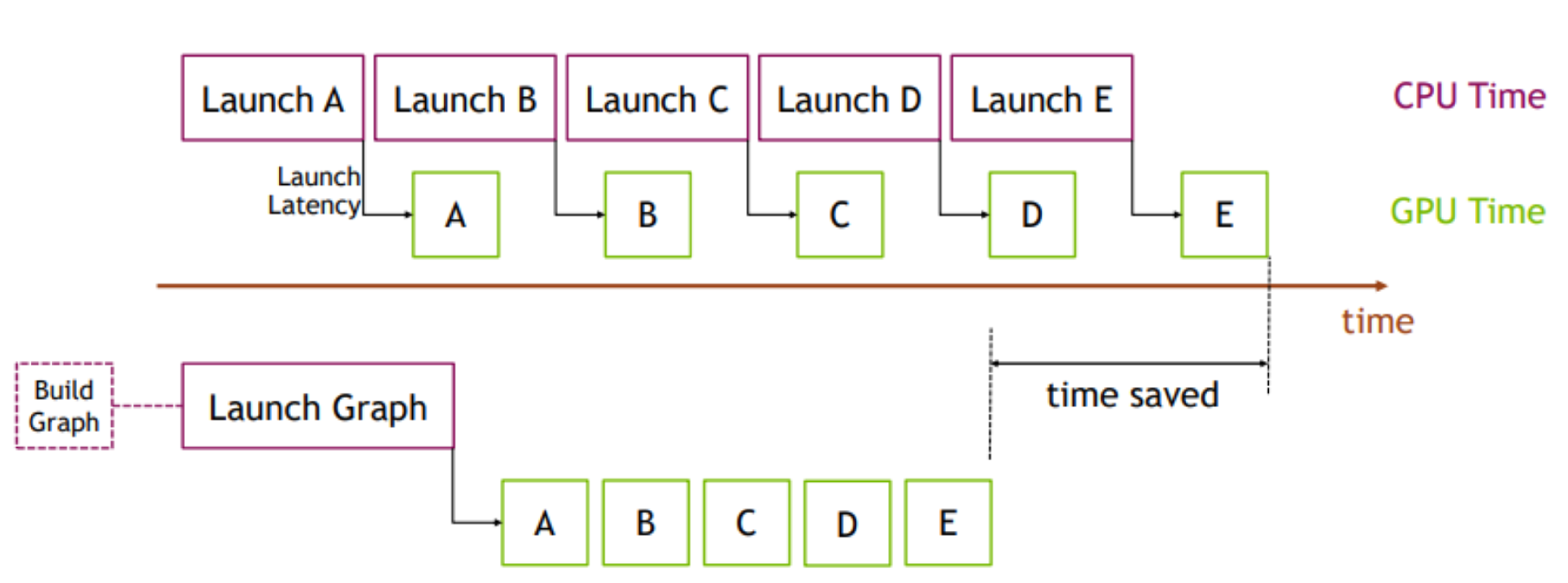
On the GPU, repeatedly launching many tiny kernels can dominate runtime. Warp supports CUDA graph capture, which records the exact sequence of kernel launches inside simulate() once, so we can replay the whole batch with a single call.

# CUDA graphs capture the exact buffers used inside simulate().
# Do not reallocate state_0/state_1 after capture.
graph = None
if wp.get_device().is_cuda:
    with wp.ScopedCapture() as capture:
        simulate()
    graph = capture.graph
    print("CUDA graph captured")
else:
    print("Running on CPU; graph capture skipped")

Warning

Graph capture records the exact memory buffers used during capture. Do not reallocate state_0 or state_1 after you capture the graph, or the replay will operate on stale memory.

Once captured, replay the graph with wp.capture_launch(graph) instead of calling simulate(). Let’s compare the two approaches with Warp’s ScopedTimer:

with wp.ScopedTimer("without_graph_capture"):
    for _ in range(120):
        simulate()

with wp.ScopedTimer("with_graph_capture"):
    for _ in range(120):
        wp.capture_launch(graph)

On a GPU you should see the graph-capture loop run meaningfully faster, because it removes most of the per-launch Python and driver overhead.

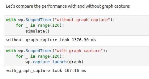
Example ScopedTimer output from one run: 120 iterations took roughly 1376 ms without graph capture and roughly 167 ms with it. Absolute numbers vary by GPU, but graph capture is consistently faster.

Complete Script

Here’s everything from this lesson assembled into one self-contained script. Download lesson1_core_concepts.py, or save the script below as lesson1_core_concepts.py in the launchable environment (see Getting Started). Open http://localhost:8080 in a browser tab first, then run the pinned uv command from the setup guide and reload the tab when Viser starts.

Show the complete runnable script

"""Newton Fundamentals - Lesson 1: Core concepts, first simulation, CUDA graphs.

Run:  python lesson1_core_concepts.py
Before running, open http://localhost:8080 in a browser tab and reload it when
the Viser server starts.
"""

import time

import numpy as np  # noqa: F401  (imported for parity with later lessons)
import warp as wp

import newton

wp.config.quiet = True


def make_viewer(name: str):
    """Open a Viser web viewer; it prints a URL (normally http://localhost:8080)."""
    return newton.viewer.ViewerViser(verbose=False)


# 1) Build a minimal scene: ground plane, one box, one sphere.
builder = newton.ModelBuilder()
builder.add_ground_plane()

box_body = builder.add_body(xform=wp.transform(wp.vec3(0.0, -1.0, 1.0), wp.quat_identity()))
builder.add_shape_box(box_body, hx=0.15, hy=0.15, hz=0.15)

sphere_body = builder.add_body(xform=wp.transform(wp.vec3(0.0, 1.0, 1.2), wp.quat_identity()))
builder.add_shape_sphere(sphere_body, radius=0.18)

print(f"Bodies: {builder.body_count}, Shapes: {builder.shape_count}")

# 2) Finalize into a device-ready Model and allocate simulation buffers.
model = builder.finalize()
state_0 = model.state()
state_1 = model.state()
control = model.control()
collision_pipeline = newton.CollisionPipeline(model)
contacts = collision_pipeline.contacts()
print(f"Model device: {model.device}, Body count: {model.body_count}")

# 3) Create a solver and define the stepping loop.
solver = newton.solvers.SolverXPBD(model, iterations=10)

fps = 60
frame_dt = 1.0 / fps
sim_substeps = 8
sim_dt = frame_dt / sim_substeps


def simulate():
    global state_0, state_1
    for _ in range(sim_substeps):
        state_0.clear_forces()
        collision_pipeline.collide(state_0, contacts)
        solver.step(state_in=state_0, state_out=state_1, control=control, contacts=contacts, dt=sim_dt)
        state_0, state_1 = state_1, state_0


# 4) Open a live viewer and log the drop.
viewer = make_viewer("01_simple_scene")
viewer.set_model(model)

print("Simulating (the first run compiles CUDA kernels, this can take a minute)...")
sim_time = 0.0
for _ in range(180):
    simulate()
    viewer.begin_frame(sim_time)
    viewer.log_state(state_0)
    viewer.end_frame()
    sim_time += frame_dt

# 5) Accelerate with CUDA graph capture (GPU only) and compare timings.
graph = None
if wp.get_device().is_cuda:
    with wp.ScopedCapture() as capture:
        simulate()
    graph = capture.graph
    print("CUDA graph captured")
else:
    print("Running on CPU; graph capture skipped")

with wp.ScopedTimer("without_graph_capture"):
    for _ in range(120):
        simulate()

if graph is not None:
    with wp.ScopedTimer("with_graph_capture"):
        for _ in range(120):
            wp.capture_launch(graph)

print("Simulation finished. Reload the pre-opened viewer tab; press Ctrl+C to exit.")
try:
    while viewer.is_running():
        time.sleep(0.1)
except KeyboardInterrupt:
    pass
viewer.close()  # stops the viser server and frees the port

Key Takeaways

You now understand the Newton pipeline end to end: a ModelBuilder assembles a scene, finalize() compiles it into a device-ready Model, and a Solver advances State using Control and Contacts one dt at a time. You also saw how CUDA graph capture collapses many kernel launches into a single replayable call for a real speedup. In the next lesson, we’ll swap our toy shapes for a real robot and start driving its joints.