DepthToSpace#
Overview#
DepthToSpace squeezes the depth dimension and moves the squeezed elements into both the width and height dimensions. Depth here is synonymous with the channel dimension, and these terms are used interchangeably. After performing the DepthToSpace operation, the total number of elements remains the same. The output width and height dimensions are both enlarged by a ratio, known as the block size parameter of the DepthToSpace operation. The reverse operation is called SpaceToDepth. More information can be found in [1].
DepthToSpace can be conceptually shown by the following NumPy code snippet. input is a NumPy array of size \(channel*height*width\). Unless explicitly stated otherwise, the channel, height, and width refer to the input dimensions in this document. The output dimension is \(1*(channel/blocksize^2)*(height*blocksize)*(width*blocksize)\). The number of channels should be a multiple of \(blocksize^2\).
import numpy as np
tmp = np.reshape(input, [blocksize, blocksize, channel // (blocksize**2), height, width])
tmp = np.transpose(tmp, [2, 3, 0, 4, 1])
output = np.reshape(tmp, [channel // (blocksize**2), height * blocksize, width * blocksize])
Reference Implementation#
TensorFlow’s depth_to_space API is used as the reference code to generate the golden output. By using this single API, the risk of misuse is minimized. In the following code snippet, both “input” and “output” are TensorFlow tensors in NCHW layout.
import tensorflow as tf
output = tf.nn.depth_to_space(input, block_size=blocksize, data_format="NCHW")
This API can also be used to generate the mapping table, as mapping table generation can be thought of as performing the DepthToSpace operation on a \(1*(blocksize^2)*tileY*tileX\) sized tensor, whose buffer is filled with an iota sequence [2] of uint16_t type. More details are covered in Tiling Method.
However, TensorFlow’s API cannot be called during runtime within the PVA solutions. Therefore, the above-generated golden output and mapping table can only be used for offline comparison. The runtime generation of the reference output and mapping table uses the NVCV API. More details are covered in Mapping Table Calculation.
Implementation Details#
Design Requirements#
Block size supports 2, 3, 4.
Data type supports
uint8_t,int8_t.Layout supports NCHW.
Supports arbitrary tensor size.
Determines the tile size and generates the mapping table during runtime.
DLUT Adoption#
Although there are various parallel VPU lookup instructions, these instructions require having correspondingly many tables to avoid memory bank conflicts. These tables are sometimes replications of one table and sometimes different tables, depending on the application. Table lookup parallelism is constrained by the memory footprint taken up by the parallel tables.
One of the main advantages of the DLUT is that it can handle bank conflicts itself. For the DepthToSpace operator, DLUT is configured to be in 1D lookup mode. Given the input size, a lookup table can be calculated beforehand and then fed to the DLUT to permute the input in an arbitrary pattern. Since the DLUT can only operate on a chunk of elements per call, the input needs to be divided into several smaller parts and use the DMA dataflow to handle the transfer and processing collaboratively, which will be covered in the next section. Note also that the DLUT can operate concurrently and independently with the VPU, but the DepthToSpace operator cannot leverage this since there is no VPU computation task in parallel to the DLUT.
Tiling Method#
If the input and output sizes fit into the VMEM allocation, one single DLUT call can permute all the elements, and no tiling is needed. Appropriate tiling methods are needed for larger input sizes. The current tiling method divides the input height and width into \(height/tileY*width/tileX\) pieces, each having a \(tileY*tileX\) shape. It further divides the input channel dimension into \(channel/blocksize^2\) pieces. Each input tile is of the dimension \(blocksize^2*tileY*tileX\). After the DepthToSpace operation, the output tile is of the dimension \(1*(tileY*blocksize)*(tileX*blocksize)\). The following figure gives a simple example, where input \(channel=8, height=2, width=2, blocksize=2\) and \(tileX=1, tileY=1\). Each colored square represents an element. We use GSDF to transfer both the input and output tiles.
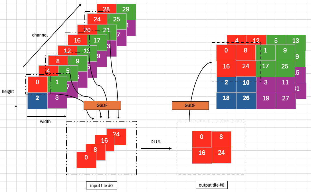
Figure 1: Tiling Example of 1x8x2x2 Input with Block Size = 2#
Maximum Tile Size#
In general, larger tile sizes have better performance due to: 1. Control logic overhead is approximately the same on a per-transfer basis, and larger tile sizes mean fewer total tiles. 2. Larger tiles usually have higher buffer utilization.
The current implementation uses uint16_t as the DLUT’s index table’s entry type, which can represent a maximum of 65536 elements, resulting in a maximum input and output size of 64KiB. There are some stack variables and separate global variables (e.g., dataflow’s triggers or handlers) that need to reside in the VMEM. Therefore, the actual size is 128KiB subtracted by this amount, and we use 8KiB within the current implementation. After that, a total of 120KiB is further divided into a PINGPONG buffer for DLUT’s input and output, with each having 60KiB. This 60KiB needs to accommodate either the input tile or the output tile. In other words, the tiling constraint is to let \(tileX\) and \(tileY\) pair that satisfies \(tileX*tileY*blocksize^2 \le 60*1024\). An illustration is shown below.
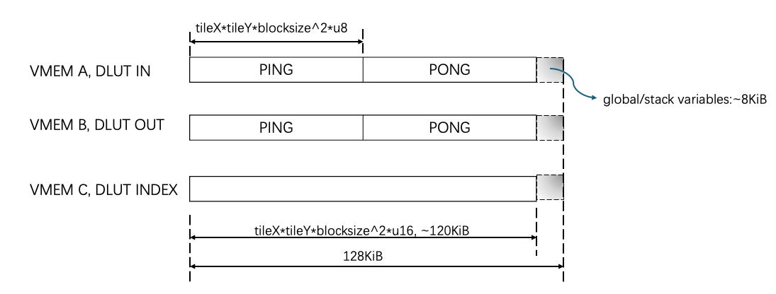
Figure 2: VMEM Allocations#
Optimum Tiling Size Determination#
The following steps are performed:
If the input tensor size is small enough to fit into the VMEM as a whole, then no tiling is needed.
Otherwise, if the input tensor’s width, height, channel, and blocksize combination belongs to one of the pre-calculated cases, just use the pre-calculated tile size.
Otherwise, use the following sub-steps:
Factor both the input tensor’s width and height into prime factors. For example, the number 100 will be factored as {1,2,2,5,5}.
Generate the full combination of factors of the width and height. For example, if \(width=100\) and \(height=50\), it will generate a candidate set in the format of {tileX, tileY}, e.g., {1, 1}, {1, 2},…,{100, 50}.
Remove an element within the candidate set if \(blocksize^2*tileX*tileY>60*1024\). If the candidate set is empty after removal, then this heuristic algorithm fails.
Sort the candidate set in descending order, by firstly comparing tile size, i.e., \(tileX*tileY\) and secondly comparing the tileX if the two have the same tile size.
Select the maximum element from the sorted candidate set and use it as the tile size.
Note that profiling on the silicon is still needed for manual checking, as there is currently no cycle-accurate model to evaluate the performance in the native mode. The simple heuristic may fail or deviate significantly from the real performance statistics. A possible scenario is that either the width or height is a relatively large prime number, so that even {1, height} or {width, 1} will let \(blocksize^2*tileX*tileY>60*1024\) fail, which results in only \(tileX=1 \land tileY=1\) left in the candidate set. This will then require manual tiling, e.g., dividing the width and height into unequal tiles.
Mapping Table Calculation#
If \(tileX=1 \land tileY=1\), the mapping table is an iota sequence starting from zero. The following code snippet is used to generate the index sequence:
// Generate the mapping table with an iota sequence: 0, 1, 2,...,((blocksize^2)*(tileY)*(tileX)-1)

// points to some valid address
uint16_t *mappingTblDevPtrHost{nullptr};
std::iota(mappingTblDevPtrHost, mappingTblDevPtrHost + blocksize * blocksize * tileY * tileX, 0);
Otherwise, NVCV APIs are used to generate the mapping table. The implementation is conceptually the same as the NumPy reference code, with the following steps:
Construct a NVCVTensorData object with dimension {blocksize, blocksize, 1, tileY, tileX}. It contains a NVCVTensorBuffer object filled with an iota sequence of uint16_t type. This sequence will be used as the mapping table after permutation.
Construct a NVCVTensorLayout object with the layout to be permuted as {1, tileY, blocksize, tileX, blocksize}.
Use nvcvTensorShapePermute API to permute both the above NVCVTensorLayout object and the strides member within the NVCVTensorBuffer object, as there is no NVCV API to permute the shape and strides simultaneously.
Traverse the elements within the NVCVTensorBuffer object using the permuted shape and strides. The traversed sequence value is the desired output. This is similar to PyTorch’s contiguous function. To be detailed, a tensor has both the physical layout and the logical layout, by manipulating the tensor’s shape and stride.
Performance#
InputTensorShape(CHW) |
DataType |
BlockSize |
Execution Time |
Submit Latency |
Total Power |
|---|---|---|---|---|---|
4x128x128 |
U8 |
2 |
0.040ms |
0.017ms |
11.831W |
4x1024x1024 |
U8 |
2 |
0.565ms |
0.022ms |
12.632W |
36x368x640 |
U8 |
3 |
1.546ms |
0.029ms |
12.032W |
16x2048x2048 |
U8 |
4 |
12.609ms |
0.036ms |
11.548W |
For detailed information on interpreting the performance table above and understanding the benchmarking setup, see Performance Benchmark.