ImageResize#
Overview#
The ImageResize operator changes the image width and height by stretching/squeezing the image pixels. A wide range of combinations of input and output image sizes is supported. The resize scale factors can be any real numbers within the Limitations mentioned below.
Two kinds of interpolation methods are available: nearest neighbor (NN), and bilinear interpolation (BL).
The list of image formats supported in the current implementation are: RGB, RGBA, NV12, U8 and U16, just as an example. The implementation is general enough to support other image formats with minor changes in parameters.
Implementation#
The ImageResize operation considers that whole coordinates fall on pixel centers. Specifically speaking, denote the input image width and height to be \(W_0\) and \(H_0\), and the output image width and height to be \(W_1\) and \(H_1\). The output pixel at indices \((j_x, j_y)\) has coordinates in the scale of input image as \(\left((j_x + 0.5) * \frac{W_0}{W_1}, (j_y+0.5)*\frac{H_0}{H_1}\right)\).
For nearest neighbor, the nearest input pixel indices are calculated as:
Here, \(NN\left[\cdot\right]\) gets the nearest integer for the real number. The output pixel value at indices \((j_x, j_y)\) equals to the input pixel value at indices \((i_x, i_y)\).
For bilinear interpolation, in each of X and Y directions we determine two adjacent indices where the fractional coordinate falls between their pixel centers:
where \(\text{floor}\left[\cdot\right]\) gets the floor integer, which is the largest integer value no greater than the real number. Values at the 4 indices \((i_x, i_y)\), \((i_x + 1, i_y)\), \((i_x, i_y + 1)\), and \((i_x + 1, i_y + 1)\) on the input image are then utilized to do bilinear interpolation.
For upsampling, the involved input indices can exceed the image range, in which case we extend the boundary values to out-of-range pixels.
For image formats with two planes like NV12, the resize operation is applied to each plane independently.
Limitations#
The scale factors for resizing images, defined as (\(R_x = W_0/W_1\)) for the width and (\(R_y = H_0/H_1\)) for the height, must not exceed 3. This limitation applies specifically to downsampling scenarios, where the original dimensions are reduced. However, when upsampling, where dimensions are increased, there is no upper limit imposed on the scale factors. The restriction arises from limited VMEM buffer capacity. Nevertheless, in most applications, both downsampling and upsampling scale factors do not exceed 3, falling within the scope of the current implementation.
Another limitation is that the input and output image sizes must be larger than 64x64. The implementation employs tiling on the output image, which is explained in detail in the next section, and the smallest tile size allowed is 32x32. For upsampling, the input GatherScatterDataFlow (GSDF) data flow achieves the boundary-pixel-extension (BPE) for out of the range pixels by padding, but padding on both sides of one direction (i.e., both left and right, or both top and bottom) is not supported. So there must be at least 2 tiles in each direction. For image format NV12, the UV plane for an image of size 64x64 is of size 32x32, which has only one tile and is unfavorable. Consequently, the output image is required to be larger than 64x64. Meanwhile, when the input image is too small, it could also cause padding on both sides of one direction in a tile. We therefore give a universal condition that both input and output image be larger than 64x64. Again, this condition is satisfied by most practical usages.
Tiling on Output#
Tiling is adopted on the output image by RasterDataFlow (RDF). For each output tile, the range of input pixel indices required for interpolation is calculated, and then GSDF is applied to read only the necessary pixels by flexible offsets and tile sizes, as well as add padding by BPE if needed.
For image formats with multiple planes, the resize operation is done independently for each plane, and each plane has its own GSDF read and RDF write data flows. For multi-channel input/output in each plane, the pixel values are interleaved in the channel dimension (i.e. HWC layout).
CupvaSampler Configuration#
The resize operation of each tile is carried out by CupvaSampler.
Nearest Neighbor by CupvaSamplerIndices2D#
For nearest neighbor, the CupvaSamplerIndices2D interface is utilized for 2D lookup with rounding
for fractional indices. The indices must be precomputed and provided.
Bilinear Interpolation by CupvaSamplerTiles#
For bilinear interpolation, the CupvaSamplerTiles interface is applied
for 2D linear interpolation with auto-index generation.
The fractional indices are generated internally.
Reduce Bank Conflicts#
The performance of CupvaSampler depends on the amount of bank conflicts,
which is highly associated with the line pitch of its input.
We align the input line pitch to \(32k + 2\) for bilinear interpolation,
so that there is no bank conflict for the adjoining 4 points used in the interpolation of one pixel.
This line pitch has empirically shown good performance for most scales.
Fractional Coordinate Generation#
Within each tile, the fractional coordinates of output pixels to be interpolated are represented as:
In the above, the step sizes equal to the scale factors \(\text{step}_x = R_x\) and \(\text{step}_y = R_y\), and the offsets are the relative coordinates of the first point in the tile.
For the CupvaSamplerIndices2D interface, fractional coordinates above are manually generated.
It can be clearly seen from (5), (6)
that coordinates of each tile are merely different in the offsets.
As 2D lookup supports shifting indices by constant offsets,
we generate the fractional coordinates of one tile with offsets 0 in advance,
and only update the offsets later for each tile.
For the CupvaSamplerTiles interface,
we only need to provide the transformation matrix
\(\left[\text{offset}_x, \text{offset}_y, \text{step}_x, \text{step}_y\right]\),
and the fractional coordinates are generated internally.
Two Levels of Fixed-Point Representation#
Fixed-point representation is employed for fractional coordinates.
Within each tile, we use Q.16 as that is the highest
fractional bits supported by CupvaSampler.
However, if Q.16 is used throughout the computations in
(1), (2), (3), (4),
error in the fractional coordinate accumulates to be on the scale of
\(\max(W_1, H_1) * 2^{-16}\), and propagates in the interpolation step to
\(\max(W_1, H_1) * 2^{-16}*V_{max}\), where \(V_{max}\) is the maximum pixel value.
The total error could become significant for large image sizes.
To tackle this issue, we use Q.32 to calculate the starting indices of each tile.
Q.32 is chosen as it is large enough for the tile start error to be less than \(2^{-16}\),
so that error from the tile start is negligible compared with the error from Q.16 in CupvaSampler.
Pre/Post Processing#
Multi-channel Inputs#
For multi-channel inputs (RGB, RGBA, the UV plane of NV12), pixel values are interleaved in the channel dimension, but the interpolation has to be done for a single channel. Therefore, we introduce pre and post processing steps to split and merge channels. The procedure for resizing a multi-channel input is as follows:
Split channels of the input image by transpose load, resulting into transposed single-channel images;
For each channel, do sampling on the transposed input to get the transposed output;
Merge the transposed single-channel outputs by transpose store.
When conducting sampling on the transposed image, parameters for X and Y directions in the transformation matrix have to be switched: \(\left[\text{offset}_y, \text{offset}_x, \text{step}_y, \text{step}_x\right]\).
Buffers with transpose load/store must have line pitch aligned to \(64k+2\).
Promotion/Demotion for Auto-index Generation#
For bilinear interpolation with auto-index generation,
the CupvaSamplerTiles interface does not support input of U8 data types (U8, RGB, RGBA, NV12),
for which we promote the input pixel values from U8 to U16 before calling the sampler
and demote from U16 to U8 for sampling results.
For multi-channel inputs, the promotion/demotion are combined with splitting/merging channels in pre/post processing kernel functions.
Details for the pre- and post-processing steps are illustrated in the following figure:
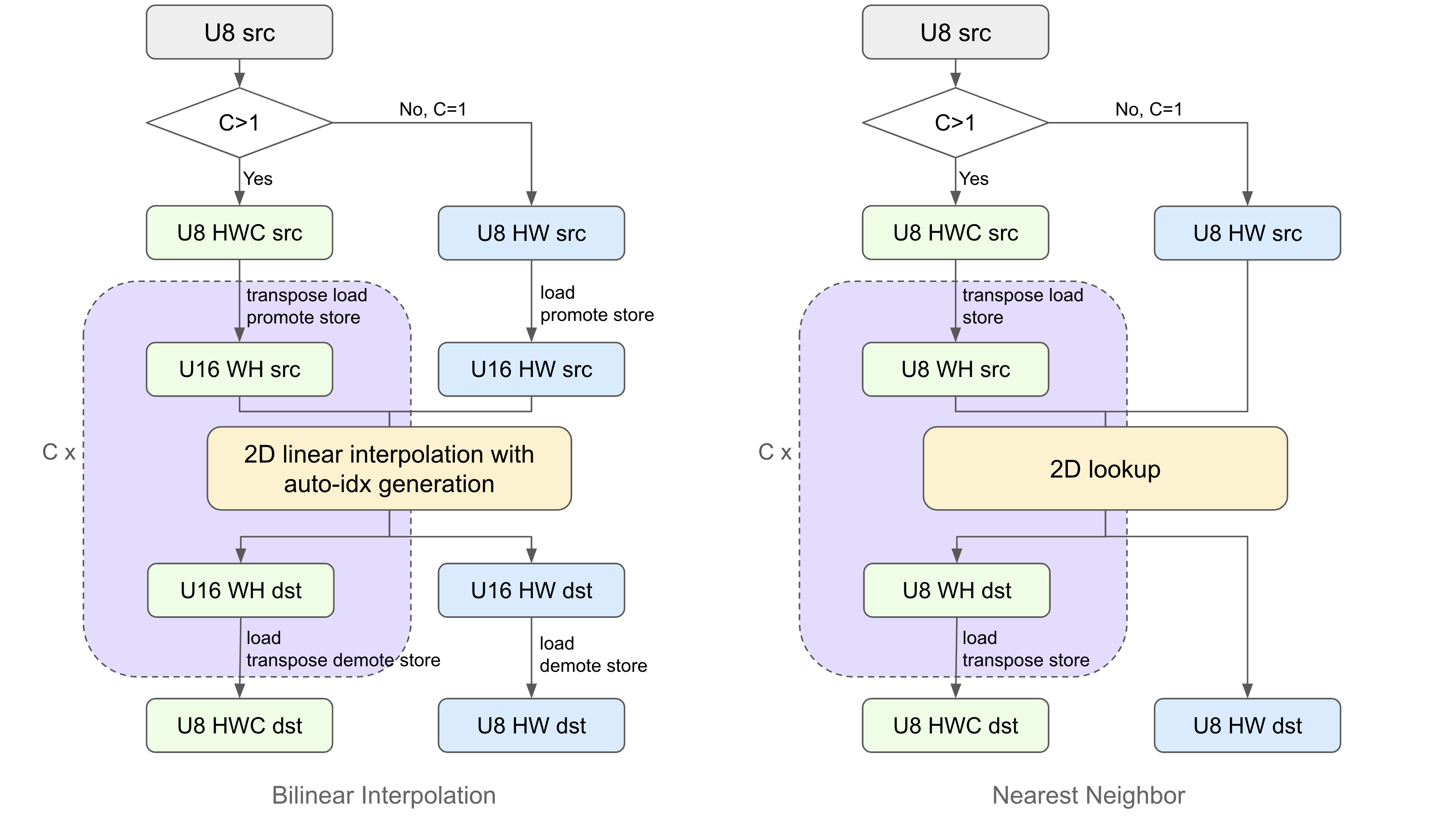
Figure 1: flow chart for U8 data type images, bilinear interpolation and nearest neighbor#
Dynamic tile size#
Since the implementation covers multiple image formats with different channel numbers (proportion of buffers are different), a wide range of scale factors, and two interpolation methods with different auxiliary buffers, it is almost impossible to find a unified VMEM allocation that obtain high DMA efficiency for all scenarios. Moreover, performance of downsampling is bounded by the DMA latency, so better DMA efficiency can greatly affects the overall performance.
Accordingly, we design an optimization mechanism to calculate the best output tile size dynamically. The function first gets the optimal VMEM buffer allocation for the given image format determined in advance, and then check all conditions for a feasible tile size:
Tile width and height must be less than 256 pixels, required by the auto-index generation mode of
CupvaSampler;Tile width is better 64B aligned, to improve VDB efficiency in the DMA write data flow;
Tile height is aligned to 32 rows, to facilitate the pre and post processing kernels;
Check the input/output buffer size: for multi-channel input/output, line pitches are aligned to \(64k+2\) for transpose load/store;
Check the pre/post processing buffer size if pre/post processing exists: line pitch of the pre-processing buffer for bilinear interpolation is aligned to \(32k+2\);
Check the RDF padding size: if the output image size is not a multiple of the output tile size, padding size in the last column/row tile must be smaller than 256.
The optimization goal is to minimize the number of tiles, in order to get a relative large tile size and reduce the GSDF trigger overhead. This optimization goal is justified by satisfactory performance in practice.
The smallest output tile size allowed is 32x32, in terms of pixels. Since the input/output tile is interleaved in the channel dimension, the actual tile width is the calculated tile width times the channel number.
Performance#
ResizeType |
ImageFormat |
InputImageSize |
OutputImageSize |
Execution Time |
Submit Latency |
Total Power |
|---|---|---|---|---|---|---|
NN |
U8 |
480x320 |
1920x1080 |
0.312ms |
0.022ms |
12.032W |
NN |
U8 |
1920x960 |
3840x2160 |
1.084ms |
0.022ms |
12.815W |
NN |
U8 |
1920x1080 |
1920x1080 |
0.313ms |
0.020ms |
13.016W |
NN |
U8 |
2880x1620 |
960x540 |
0.295ms |
0.016ms |
13.044W |
NN |
U8 |
3840x2160 |
1920x960 |
0.496ms |
0.021ms |
13.627W |
NN |
U16 |
480x320 |
1920x1080 |
0.345ms |
0.021ms |
13.098W |
NN |
U16 |
1920x960 |
3840x2160 |
1.184ms |
0.024ms |
14.091W |
NN |
U16 |
1920x1080 |
1920x1080 |
0.350ms |
0.021ms |
14.493W |
NN |
U16 |
2880x1620 |
960x540 |
0.580ms |
0.017ms |
12.842W |
NN |
U16 |
3840x2160 |
1920x960 |
1.067ms |
0.020ms |
13.428W |
NN |
RGB8 |
480x320 |
1920x1080 |
0.976ms |
0.023ms |
11.831W |
NN |
RGB8 |
1920x960 |
3840x2160 |
3.923ms |
0.022ms |
12.032W |
NN |
RGB8 |
1920x1080 |
1920x1080 |
1.253ms |
0.023ms |
11.932W |
NN |
RGB8 |
2880x1620 |
960x540 |
1.321ms |
0.020ms |
13.116W |
NN |
RGB8 |
3840x2160 |
1920x960 |
2.623ms |
0.024ms |
12.331W |
NN |
RGBA8 |
480x320 |
1920x1080 |
1.265ms |
0.026ms |
11.731W |
NN |
RGBA8 |
1920x960 |
3840x2160 |
5.148ms |
0.024ms |
11.932W |
NN |
RGBA8 |
1920x1080 |
1920x1080 |
1.624ms |
0.023ms |
11.932W |
NN |
RGBA8 |
2880x1620 |
960x540 |
1.670ms |
0.020ms |
12.815W |
NN |
RGBA8 |
3840x2160 |
1920x960 |
3.342ms |
0.025ms |
12.231W |
NN |
NV12 |
480x320 |
1920x1080 |
0.555ms |
0.021ms |
11.447W |
NN |
NV12 |
1920x960 |
3840x2160 |
2.039ms |
0.027ms |
12.032W |
NN |
NV12 |
1920x1080 |
1920x1080 |
0.604ms |
0.021ms |
12.231W |
NN |
NV12 |
2880x1620 |
960x540 |
0.562ms |
0.018ms |
13.016W |
NN |
NV12 |
3840x2160 |
1920x960 |
1.005ms |
0.021ms |
13.116W |
LINEAR |
U8 |
480x320 |
1920x1080 |
0.317ms |
0.021ms |
11.831W |
LINEAR |
U8 |
1920x960 |
3840x2160 |
1.229ms |
0.023ms |
12.03W |
LINEAR |
U8 |
1920x1080 |
1920x1080 |
0.412ms |
0.021ms |
12.13W |
LINEAR |
U8 |
2880x1620 |
960x540 |
0.388ms |
0.015ms |
13.51W |
LINEAR |
U8 |
3840x2160 |
1920x960 |
0.720ms |
0.021ms |
13.116W |
LINEAR |
U16 |
480x320 |
1920x1080 |
0.330ms |
0.020ms |
13.098W |
LINEAR |
U16 |
1920x960 |
3840x2160 |
1.217ms |
0.023ms |
13.498W |
LINEAR |
U16 |
1920x1080 |
1920x1080 |
0.334ms |
0.020ms |
15.359W |
LINEAR |
U16 |
2880x1620 |
960x540 |
0.561ms |
0.017ms |
13.044W |
LINEAR |
U16 |
3840x2160 |
1920x960 |
0.898ms |
0.021ms |
13.627W |
LINEAR |
RGB8 |
480x320 |
1920x1080 |
0.904ms |
0.025ms |
11.731W |
LINEAR |
RGB8 |
1920x960 |
3840x2160 |
3.803ms |
0.023ms |
11.831W |
LINEAR |
RGB8 |
1920x1080 |
1920x1080 |
1.213ms |
0.023ms |
11.932W |
LINEAR |
RGB8 |
2880x1620 |
960x540 |
1.137ms |
0.020ms |
13.4W |
LINEAR |
RGB8 |
3840x2160 |
1920x960 |
2.950ms |
0.023ms |
12.132W |
LINEAR |
RGBA8 |
480x320 |
1920x1080 |
1.253ms |
0.025ms |
11.731W |
LINEAR |
RGBA8 |
1920x960 |
3840x2160 |
5.138ms |
0.025ms |
11.932W |
LINEAR |
RGBA8 |
1920x1080 |
1920x1080 |
1.616ms |
0.023ms |
11.932W |
LINEAR |
RGBA8 |
2880x1620 |
960x540 |
1.761ms |
0.021ms |
12.331W |
LINEAR |
RGBA8 |
3840x2160 |
1920x960 |
3.773ms |
0.024ms |
12.032W |
LINEAR |
NV12 |
480x320 |
1920x1080 |
0.481ms |
0.023ms |
11.831W |
LINEAR |
NV12 |
1920x960 |
3840x2160 |
1.885ms |
0.026ms |
12.032W |
LINEAR |
NV12 |
1920x1080 |
1920x1080 |
0.659ms |
0.024ms |
12.032W |
LINEAR |
NV12 |
2880x1620 |
960x540 |
0.655ms |
0.017ms |
12.915W |
LINEAR |
NV12 |
3840x2160 |
1920x960 |
1.184ms |
0.023ms |
13.199W |
For detailed information on interpreting the performance table above and understanding the benchmarking setup, see Performance Benchmark.