Train With Mixed Precision
Abstract
Mixed precision methods combine the use of different numerical formats in one computational workload. This document describes the application of mixed precision to deep neural network training.
There are numerous benefits to using numerical formats with lower precision than 32-bit floating point. First, they require less memory, enabling the training and deployment of larger neural networks. Second, they require less memory bandwidth which speeds up data transfer operations. Third, math operations run much faster in reduced precision, especially on GPUs with Tensor Core support for that precision. Mixed precision training achieves all these benefits while ensuring that no task-specific accuracy is lost compared to full precision training. It does so by identifying the steps that require full precision and using 32-bit floating point for only those steps while using 16-bit floating point everywhere else.
Mixed precision training offers significant computational speedup by performing operations in half-precision format, while storing minimal information in single-precision to retain as much information as possible in critical parts of the network. Since the introduction of Tensor Cores in the Volta and Turing architectures, significant training speedups are experienced by switching to mixed precision -- up to 3x overall speedup on the most arithmetically intense model architectures. Using mixed precision training requires two steps:
- Porting the model to use the FP16 data type where appropriate.
- Adding loss scaling to preserve small gradient values.
The ability to train deep learning networks with lower precision was introduced in the Pascal architecture and first supported in CUDA 8 in the NVIDIA Deep Learning SDK.
Mixed precision is the combined use of different numerical precisions in a computational method.
Half precision (also known as FP16) data compared to higher precision FP32 vs FP64 reduces memory usage of the neural network, allowing training and deployment of larger networks, and FP16 data transfers take less time than FP32 or FP64 transfers.
Single precision (also known as 32-bit) is a common floating point format (float in C-derived programming languages), and 64-bit, known as double precision (double).
Deep Neural Networks (DNNs) have led to breakthroughs in a number of areas, including:
- image processing and understanding
- language modeling
- language translation
- speech processing
- game playing, and many others.
DNN complexity has been increasing to achieve these results, which in turn has increased the computational resources required to train these networks. One way to lower the required resources is to use lower-precision arithmetic, which has the following benefits.
- Half-precision floating point format (FP16) uses 16 bits, compared to 32 bits for single precision (FP32). Lowering the required memory enables training of larger models or training with larger mini-batches.
- Execution time can be sensitive to memory or arithmetic bandwidth. Half-precision halves the number of bytes accessed, thus reducing the time spent in memory-limited layers. NVIDIA GPUs offer up to 8x more half precision arithmetic throughput when compared to single-precision, thus speeding up math-limited layers.
Figure 1. Training curves for the bigLSTM English language model shows the benefits of the mixed-precision training techniques. The Y-axis is training loss. Mixed precision without loss scaling (grey) diverges after a while, whereas mixed precision with loss scaling (green) matches the single precision model (black).
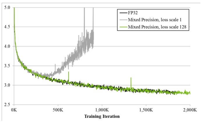
Since DNN training has traditionally relied on IEEE single-precision format, this guide will focus on how to train with half precision while maintaining the network accuracy achieved with single precision (as Figure 1). This technique is called mixed-precision training since it uses both single and half-precision representations.
2.1. Half Precision Format
IEEE 754 standard defines the following 16-bit half-precision floating point format: 1 sign bit, 5 exponent bits, and 10 fractional bits.
Exponent is encoded with 15 as the bias, resulting in [-14, 15] exponent range (two exponent values, 0 and 31, are reserved for special values). An implicit lead bit 1 is assumed for normalized values, just like in other IEEE floating point formats. Half precision format leads to the following dynamic range and precision:
- 2-14 to 215, 11 bits of significand
- 2-24 to 2-15, significand bits decrease as the exponent gets smaller. Exponent k in [-24, -15] range results in (25 - k) bits of significand precision.
Some example magnitudes:
- 65,504
- 2-14= ~6.10e-5
- 2-24= ~5.96e-8
Half precision dynamic range, including denormals, is 40 powers of 2. For comparison, single precision dynamic range including denormals is 264 powers of 2.
2.2. Tensor Core Math
The Volta generation of GPUs introduces Tensor Cores, which provide 8x more throughput than single precision math pipelines. Each Tensor Core performs D = A x B + C, where A, B, C, and D are matrices. A and B are half precision 4x4 matrices, whereas D and C can be either half or single precision 4x4 matrices. In other words, Tensor Core math can accumulate half precision products into either single or half precision outputs.
In practice, higher performance is achieved when A and B dimensions are multiples of 8. cuDNN v7 and cuBLAS 9 include some functions that invoke Tensor Core operations, for performance reasons these require that input and output feature map sizes are multiples of 8. For more information, see the NVIDIA cuDNN Developer Guide.
The reason half precision is so attractive is that the V100 GPU has 640 Tensor Cores, so they can all be performing 4x4 multiplications all at the same time. The theoretical peak performance of the Tensor Cores on the V100 is approximately 120 TFLOPS. This is about an order of magnitude (10x) faster than double precision (FP64) and about four times faster than single precision (FP32).
Matrix multiplies are at the core of Convolutional Neural Networks (CNN). CNNs are very common in deep learning on many networks. Beginning in CUDA 9 and cuDNN 7, the convolution operations are done using Tensor Cores whenever possible. This can greatly improve the training speed as well as the inference speed of CNNs or models that contain convolutions.
2.3. Considering When Training With Mixed Precision
Assuming the framework supports Tensor Core math, simply enabling the Tensor Core path in the framework trains many networks faster. You can choose the FP16 format for tensors and/or convolution/fully-connected layers and keep all the hyperparameters of the FP32 training session. For more details, refer to Frameworks.
However, some networks require their gradient values to be shifted into FP16 representable range to match the accuracy of FP32 training sessions. The figure below illustrates one such case.
Figure 2. Histogram of activation gradient magnitudes throughout FP32 training of Multibox SSD network. The x-axis is logarithmic, except for the zero entry. For example, 66.8% of values were 0 and 4% had magnitude in the (2-32 , 2-30) range.
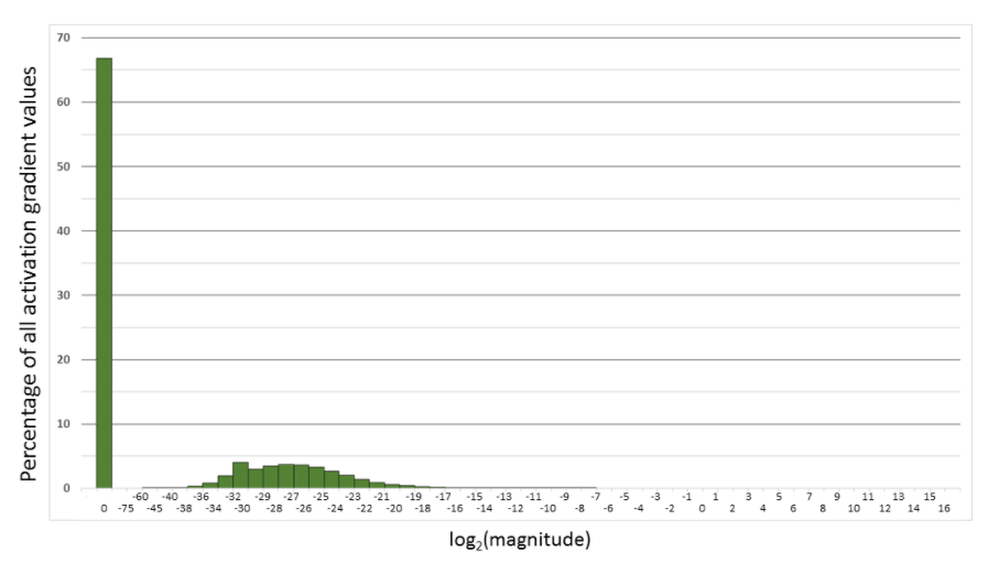
However, this isn’t always the case. You may have to do some scaling and normalization to use FP16 during training.
Figure 3. Histogram of activation gradient magnitudes throughout FP32 training of Multibox SSD network. Both x- and y-axes are logarithmic.
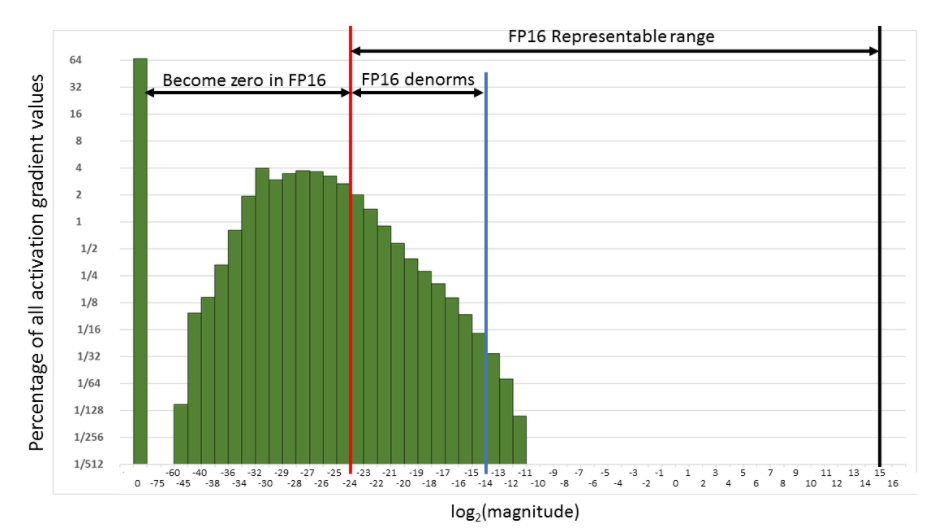
Consider the histogram of activation gradient values (shown with linear and log y-scales above), collected across all layers during FP32 training of the Multibox SSD detector network (VGG-D backbone). When converted to FP16, 31% of these values become zeros, leaving only 5.3% as nonzeros which for this network lead to divergence during training.
Much of the FP16 representable range was left unused by the gradient values. Therefore, if we shift the gradient values to occupy more of that range, we can preserve many values that are otherwise lost to 0s.
For this particular network, shifting by three exponent values (multiply by 8) was sufficient to match the accuracy achieved with FP32 training by recovering the relevant values lost to 0. Shifting by 15 exponent values (multiplying by 32K) would recover all but 0.1% of values lost to 0 when converting to FP16 and still avoid overflow. In other words, FP16 dynamic range is sufficient for training, but gradients may have to be scaled to move them into the range to keep them from becoming zeros in FP16.
2.3.1. Loss Scaling To Preserve Small Gradient Magnitudes
As was shown in the previous section, successfully training some networks requires gradient value scaling to keep them from becoming zeros in FP16. This can be achieved with a single multiplication. You can scale the loss values computed in the forward pass, before starting backpropagation. By the chain rule, backpropagation ensures that all the gradient values of the same amount are scaled. This requires no extra operations during backpropagation and keeps the relevant gradient values from becoming zeros and losing that gradient information.
Weight gradients must be unscaled before weight update, to maintain the magnitude of updates the same as in FP32 training. It is simplest to perform this descaling right after the backward pass but before gradient clipping or any other gradient-related computations. This ensures that no hyperparameters (such as gradient clipping threshold, weight decay, etc.) have to be adjusted.
While many networks match FP32 training results when all tensors are stored in FP16, some require updating an FP32 copy of weights. Furthermore, values computed by large reductions should be left in FP32. Examples of this include statistics (mean and variance) computed by batch-normalization, SoftMax. Batch-normalization can still take FP16 inputs and outputs, saving half the bandwidth compared to FP32, it’s just that the statistics and value adjustment should be done in FP32. This leads to the following high-level procedure for training:
2.3.2. Choosing A Scaling Factor
The procedure described in the previous section requires you to pick a loss scaling factor to adjust the gradient magnitudes. You can choose a large scaling factor as long as it doesn’t cause overflow during backpropagation. This would lead to weight gradients containing infinities or NaNs, which in turn would irreversibly damage the weights during the update. These overflows can be easily and efficiently detected by inspecting the computed weight gradients, for example, multiplying the weight gradient with 1/S step in the previous section.
There are several options to choose the loss scaling factor. The simplest one is to pick a constant scaling factor. We trained a number of feed-forward and recurrent networks with Tensor Core math for various tasks. The network's scaling factors ranged from 8 to 32K (many networks did not require a scaling factor). The network accuracy was achieved from training in FP32. However, since the minimum required scaling factor can depend on the network, framework, minibatch size, etc., some trial and error may be required when picking a scaling value. A constant scaling factor can be chosen more directly if gradient statistics are available. Choose a value so that its product with the maximum absolute gradient value is below 65,504 (the maximum value representable in FP16). A more robust approach is to choose the loss scaling factor dynamically. The basic idea is to start with a large scaling factor and then reconsider it in each training iteration. If no overflow occurs for a chosen number of iterations N, then increase the scaling factor. If an overflow occurs, skip the weight update and decrease the scaling factor. We found that as long as one skips updates infrequently the training schedule does not have to be adjusted to reach the same accuracy as FP32 training. Note that N effectively limits how frequently we may overflow and skip updates. The rate for scaling factor update can be adjusted by picking the increase/decrease multipliers as well as N, the number of nonoverflow iterations before the increase. We successfully trained networks with N = 2000, increasing scaling factor by 2, decreasing scaling factor by 0.5, many other settings are valid as well. Dynamic loss-scaling approach leads to the following high-level training procedure:
Using mixed precision training requires three steps:
- Converting the model to use the float16 data type where possible.
- Keeping float32 master weights to accumulate per-iteration weight updates.
- Using loss scaling to preserve small gradient values.
Frameworks that support fully automated mixed precision training also support:
- Automatic loss scaling and master weights integrated into optimizer classes
- Automatic casting between float16 and float32 to maximize speed while ensuring no loss in task-specific accuracy
In those frameworks with automatic support, using mixed precision can be as simple as adding one line of code or enabling a single environment variable. Currently, the frameworks with support for automatic mixed precision are TensorFlow, PyTorch, and MXNet. Refer to NVIDIA Automatic Mixed Precision for Deep Learning for more information, along with the Frameworks section below.
NVIDIA Tensor Cores provide hardware acceleration for mixed precision training. On a V100 GPU, Tensor Cores can speed up matrix multiply and convolution operations by up to 8x in float16 over their float32 equivalents.
Taking full advantage of Tensor Cores may require changes to model code. This section describes three steps you can take to maximize the benefit that Tensor Cores provide:
- Satisfy Tensor Core shape constraints
- Increase arithmetic intensity
- Decrease fraction of work in non-Tensor Core operations
The above benefits are ordered by increasing complexity, and in particular, the first step (satisfying shape constraints) usually provides most of the benefit for little effort.
4.1. Satisfying Tensor Core Shape Constraints
Due to their design, Tensor Cores have shape constraints on their inputs.
For matrix multiplication:
- On FP16 inputs, all three dimensions (M, N, K) must be multiples of 8.
- On INT8 inputs (Turing only), all three dimensions must be multiples of 16.
- On FP16 inputs, input and output channels must be multiples of 8.
- On INT8 inputs (Turing only), input and output channels must be multiples of 16.
In practice, for mixed precision training, our recommendations are:
- Choose mini-batch to be a multiple of 8
- Choose linear layer dimensions to be a multiple of 8
- Choose convolution layer channel counts to be a multiple of 8
- For classification problems, pad vocabulary to be a multiple of 8
- For sequence problems, pad the sequence length to be a multiple of 8
4.2. Increasing Arithmetic Intensity
Arithmetic intensity is a measure of how much computational work is to be performed in a kernel per input byte. For example, a V100 GPU has 125 TFLOPs of math throughput and 900 GB/s of memory bandwidth. Taking the ratio of the two, we see that any kernel with fewer than ~140 FLOPs per input byte will be memory-bound. That is, Tensor Cores cannot run at full throughput because memory bandwidth will be the limiting factor. A kernel with sufficient arithmetic intensity to allow full Tensor Core throughput is compute-bound.
It is possible to increase arithmetic intensity both in model implementation and model architecture. To increase arithmetic intensity in model implementation:
- Concatenate weights and gate activations in recurrent cells.
- Concatenate activations across time in sequence models.
To increase arithmetic intensity in model architecture:
- Prefer dense math operations.
- For example, vanilla convolutions have much higher arithmetic intensity than depth-wise separable convolutions.
- Prefer wider layers when possible accuracy-wise.
4.3. Decreasing Non-Tensor Core Work
Many operations in deep neural networks are not accelerated by Tensor Cores, and it is important to understand the effect this has on end-to-end speed-ups. For example, suppose that a model spends one half of the total training time in Tensor Core-accelerated operations (matrix multiplication and convolution). If Tensor Cores provide a 5x speed-up for those operations, then the total speedup will be 1. / (0.5 + (0.5 / 5.)) = 1.67x.
In general, as Tensor Core operations represent a decreasing fraction of total work, the more important it is to focus on optimizing non-Tensor Core operations. It is possible to speed-up these operations by hand, using custom CUDA implementations along with framework integration. Furthermore, frameworks are beginning to provide support for automatically speeding up non-Tensor Core ops with compiler tools. Examples include XLA for TensorFlow and the PyTorch JIT.
To take advantage of mixed precision training, ensure you meet the following minimum requirements:
Procedure
- Run on the Volta or Turing architecture.
- Install an NVIDIA Driver. Currently CUDA 10.1 is supported, which requires NVIDIA driver release 418.xx+. However, if you are running on a Tesla (Tesla V100, Tesla P4, Tesla P40, or Tesla P100), you may use the NVIDIA driver release 384.111+ or 410. The CUDA driver's compatibility package only supports particular drivers. For a complete list of supported drivers, see the CUDA Application Compatibility topic. For more information, see CUDA Compatibility and Upgrades.
- Install the CUDA® Toolkit™ .
- Install cuDNN.
Note:
If using an NVIDIA optimized framework container, that was pulled from the NGC container registry, you will still need to install an NVIDIA driver on your base operating system. However, CUDA and cuDNN will come included in the container. For more information, refer to the Frameworks Support Matrix.
Most major deep learning frameworks have begun to merge support for half precision training techniques that exploit Tensor Core calculations in Volta and Turing. Additional optimization pull requests are at various stages and listed in their respective sections.
For NVCaffe, Caffe2, MXNet, Microsoft Cognitive Toolkit, PyTorch, TensorFlow and Theano, Tensor Core acceleration is automatically enabled if FP16 storage is enabled.
While frameworks like Torch will tolerate the latest architecture, it currently does not exploit Tensor Core functionality.
PyTorch
PyTorch includes support for FP16 storage and Tensor Core math. To achieve optimum performance, you can train a model using Tensor Core math and mixed precision.
7.1.1. Automatic Mixed Precision Training In PyTorch
The automatic mixed precision feature is available starting inside the NVIDIA NGC PyTorch 19.03+ containers.
To get started, we recommend using AMP (Automatic Mixed Precision), which enables mixed precision in only 3 lines of Python. AMP is available through NVIDIA’s Apex repository of mixed precision and distributed training tools. The AMP API is documented in detail here.
7.1.2. Success Stories
The models where we have seen speedup using mixed precision are:
| Model | Speedup |
|---|---|
| NVIDIA Sentiment Analysis | 4.5X speedup |
| FAIRSeq | 3.5X speedup |
| GNMT | 2X speedup |
7.1.3. Tensor Core Optimized Model Scripts For PyTorch
The Tensor Core examples provided in GitHub focus on achieving the best performance and convergence using NVIDIA Volta Tensor Cores . It uses the latest deep learning example networks and model scripts for training.
These examples focus on achieving the best performance and convergence from NVIDIA Volta Tensor Cores by using the latest deep learning example networks for training. Each example model trains with mixed precision Tensor Cores on Volta, therefore you can get results much faster than training without Tensor Cores. This model is tested against each NGC monthly container release to ensure consistent accuracy and performance over time. This container includes the following Tensor Core examples.
7.1.4. Manual Conversion To Mixed Precision In PyTorch
We recommend using AMP to implement mixed precision in your model. However, if you wish to implement mixed precision yourself, refer to our GTC talk on manual mixed precision (video, slides).
TensorFlow
TensorFlow supports FP16 storage and Tensor Core math. Models that contain convolutions or matrix multiplications using the tf.float16 data type will automatically take advantage of Tensor Core hardware whenever possible.
In order to make use of Tensor Cores, FP32 models will need to be converted to use a mix of FP32 and FP16. This can be done either automatically using automatic mixed precision (AMP) or manually.
7.2.1. Automatic Mixed Precision Training In TensorFlow
For models already using a tf.train.Optimizer or tf.keras.optimizers.Optimizer for both compute_gradients() and apply_gradients() operations (for example, by calling optimizer.minimize() or model.fit()), automatic mixed precision can be enabled by wrapping the optimizer with tf.train.experimental.enable_mixed_precision_graph_rewrite().
Graph-based example:
            opt = tf.train.AdamOptimizer()
opt = tf.train.experimental.enable_mixed_precision_graph_rewrite(opt)
train_op = opt.miminize(loss)
Keras-based example:
            opt = tf.keras.optimizers.Adam()
opt = tf.train.experimental.enable_mixed_precision_graph_rewrite(opt)
model.compile(loss=loss, optimizer=opt)
model.fit(...)
You can also set the environment variable inside a TensorFlow Python script. Issue the following code at the beginning of the script:
os.environ['TF_ENABLE_AUTO_MIXED_PRECISION'] = '1'
When enabled, automatic mixed precision will do two things:
- Insert the appropriate cast operations into your TensorFlow graph to use float16 execution and storage where appropriate. This enables the use of Tensor Cores along with memory storage and bandwidth savings.
- Turn on automatic loss scaling inside the training Optimizer object.
For more information on automatic mixed precision, refer to the NVIDIA TensorFlow User Guide.
7.2.2. Success Stories
The models where we have seen speedup using mixed precision are:
| Model | Speedup |
|---|---|
| BERT Q&A | 3.3X speedup |
| GNMT | 1.7X speedup |
| NCF | 2.6X speedup |
| SSD-RN50-FPN-640 | 2.5X speedup |
7.2.3. Tensor Core Optimized Model Scripts For TensorFlow
The Tensor Core examples provided in GitHub focus on achieving the best performance and convergence using NVIDIA Volta Tensor Cores . It uses the latest deep learning example networks and model scripts for training.
Each example model trains with mixed precision Tensor Cores on Volta, therefore you can get results much faster than training without Tensor Cores. This model is tested against each NGC monthly container release to ensure consistent accuracy and performance over time. This container includes the following Tensor Core examples.
7.2.4. Manual Conversion To Mixed Precision Training In TensorFlow
Procedure
- Pull the latest TensorFlow container from the NVIDIA GPU Cloud (NGC) container registry. The container is already built, tested, tuned, and ready to run. The TensorFlow container includes the latest CUDA version, FP16 support, and is optimized for the latest architecture. For step-by-step pull instructions, refer to the NVIDIA Containers for Deep Learning Frameworks User Guide.
- Use the
tf.float16data type on models that contain convolutions or matrix multiplications. This data type automatically takes advantage of the Tensor Core hardware whenever possible, in other words, to increase your chances for Tensor Core acceleration, choose where possible multiple of eight linear layer matrix dimensions and convolution channel counts. For example:dtype = tf.float16 data = tf.placeholder(dtype, shape=(nbatch, nin)) weights = tf.get_variable('weights', (nin, nout), dtype) biases = tf.get_variable('biases', nout, dtype, initializer=tf.zeros_initializer()) logits = tf.matmul(data, weights) + biases
- Ensure that the trainable variables are in float32 precision and cast them to float16 before using them in the model. For example:
tf.cast(tf.get_variable(..., dtype=tf.float32), tf.float16)
float32_variable_storage_gettershown in the following example. - Ensure that the SoftMax calculation is in float32 precision. For example:
tf.losses.softmax_cross_entropy(target, tf.cast(logits, tf.float32))
- Apply loss-scaling as outlined in the previous sections. Loss scaling involves multiplying the loss by a scale factor before computing gradients, and then dividing the resulting gradients by the same scale again to re-normalize them. For example, to apply a constant loss scaling factor of 128:
            loss, params = ...
scale = 128
grads = [grad / scale for grad in tf.gradients(loss * scale, params)]
MXNet
MXNet includes support for FP16 storage and Tensor Core math. To achieve optimum performance, you need to train a model using Tensor Core math and FP16 mode on MXNet.
The following procedure is typical for when you want to have your entire network in FP16. Alternatively, you can take output from any layer and cast it to FP16. Subsequent layers will be in FP16 and will use Tensor Core math if applicable.
7.3.1. Automatic Mixed Precision Training In MXNet
The automatic mixed precision feature is available starting inside the NVIDIA NGC MXNet 19.04+ containers.
Training deep learning networks is a very computationally intensive task. Novel model architectures tend to have an increasing number of layers and parameters, which slows down training. Fortunately, new generations of training hardware as well as software optimizations make training these new models a feasible task.
Most of the hardware and software training optimization opportunities involve exploiting lower precision like FP16 in order to utilize the Tensor Cores available on new Volta and Turing GPUs. While training in FP16 showed great success in image classification tasks, other more complicated neural networks typically stayed in FP32 due to difficulties in applying the FP16 training guidelines that are needed to ensure proper model training.
That is where AMP (Automatic Mixed Precision) comes into play- it automatically applies the guidelines of FP16 training, using FP16 precision where it provides the most benefit, while conservatively keeping in full FP32 precision operations unsafe to do in FP16.
The MXNet AMP tutorial, located in /opt/mxnet/nvidia-examples/AMP/AMP_tutorial.md inside this container, shows how to get started with mixed precision training using AMP for MXNet, using by example the SSD network from GluonCV.
7.3.2. Tensor Core Optimized Model Scripts For MXNet
The Tensor Core examples provided in GitHub focus on achieving the best performance and convergence using NVIDIA Volta Tensor Cores. It also uses the latest deep learning example networks and model scripts for training.
Each example model trains with mixed precision Tensor Cores starting with the Volta architecture, therefore you can get results much faster than training without Tensor Cores. This model is tested against each NGC monthly container release to ensure consistent accuracy and performance over time. The MXNet container includes the following MXNet Tensor Core examples:
7.3.3. Manual Conversion To Mixed Precision Training In MXNet
Procedure
- Pull the latest MXNet container from the NVIDIA GPU Cloud (NGC) container registry. The container is already built, tested, tuned, and ready to run. The MXNet container includes the latest CUDA version, FP16 support, and is optimized for the latest architecture. For step-by-step pull instructions, refer to the NVIDIA Containers for Deep Learning Frameworks User Guide.
- To use the IO pipeline, use the
IndexedRecordIOformat of input. It differs from the legacyRecordIOformat, by including an additional index file with an.idxextension. The.idxfile is automatically generated when using theim2rec.pytool, to generate newRecordIOfiles. If you already have the.recfile without the corresponding.idxfile, you can generate the index file withtools/rec2idx.pytool:python tools/rec2idx.py <path to .rec file> <path to newly created .idx file>
- To use FP16 training with MXNet, cast the data (input to the network) to FP16.
mxnet.sym.Cast(data=input_data, dtype=numpy.float16)
- Cast back to FP32 before the SoftMax layer.
- If you encounter precision problems, it is beneficial to scale the loss up by 128, and scale the application of the gradients down by 128. This ensures higher gradients during the backward pass calculation, but will still correctly update the weights. For example, if out last layer is
mx.sym.SoftmaxOutput(cross-entropy loss), and the initial learning rate is 0.1, add agrad_scaleparameter:mxnet.sym.SoftmaxOutput(other_args, grad_scale=128.0)
mxnet.optimizer.SGD(other_args, rescale_grad=1.0/128)
Tip:When training in FP16, it is best to use multi-precision optimizers that keep the weights in FP32 and perform the backward pass in FP16. For example, for SGD with momentum, you would issue the following:
mxnet.optimizer.SGD(other_args, momentum=0.9, multi_precision=True)
Alternatively, you can pass
'multi_precision': Trueto theoptimizer_paramsoption in themodel.fitmethod.
Caffe2
Caffe2 includes support for FP16 storage and Tensor Core math. To achieve optimum performance, you can train a model using Tensor Core math and FP16 mode on Caffe2.
When training a model on Caffe2 using Tensor Core math and FP16, the following actions need to take place:
- Prepare your data. You can generate data in FP32 and then cast it down to FP16. The GPU transforms path of the
ImageInputoperation can do this casting in a fused manner. - Forward pass. Since data is given to the network in FP16, all of the subsequent operations will run in FP16 mode, therefore:
- Select which operators need to have both FP16 and FP32 parameters by setting the type of Initializer used. Typically, the Conv and FC operators need to have both parameters.
- Cast the output of forward pass, before SoftMax, back to FP32.
- To enable Tensor Core, pass
enable_tensor_core=TruetoModelHelperwhen representing a new model.
- Update the primary FP32 copy of the weights using the FP16 gradients you just computed. For example:
- Cast up gradients to FP32.
- Update the FP32 copy of parameters.
- Cast down the FP32 copy of parameters to FP16 for the next iteration.
- Select which operators need to have both FP16 and FP32 parameters by setting the type of Initializer used. Typically, the Conv and FC operators need to have both parameters.
- Gradient scaling.
- To scale, multiply the loss by the scaling factor.
- To descale, divide
LRandweight_decayby the scaling factor.
7.4.1. Running FP16 Training On Caffe2
Procedure
- Pull the latest Caffe2 container from the NVIDIA GPU Cloud (NGC) container registry. The container is already built, tested, tuned, and ready to run. The Caffe2 container includes the latest CUDA version, FP16 support, and is optimized starting with the Volta architecture. For step-by-step pull instructions, see the NVIDIA Containers for Deep Learning Frameworks User Guide.
- Run the following Python script with the appropriate command line arguments. You can test using the ResNet-50 image classification training script included in Caffe2.
            python caffe2/python/examples/resnet50_trainer.py --train_data
<path> --test_data <path> --num-gpus <int> --batch-size <int>
--dtype float16 --enable-tensor-core --cudnn_workspace_limit_mb
1024 --image_size 224
caffe2/python/examples/resnet50_trainer.py --help
To enhance performance, the following changes must be made:- The network definition in
caffe2/python/models/resnet.pymust be changed to reflect version 1 of the network by changing the residual block striding from the 3x3 convolution to the first 1x1 convolution operator. - Enable optimized communication operators and disable some communication ops by adding the
use_nccl=Trueandbroadcast_computed_params=Falseflags to the data_parallel_model.Parallelize call incaffe2/python/examples/resnet50_trainer.py. - Add
decode_threads=3anduse_gpu_transform=Trueto the brew.image_input call. This tweaks the amount of CPU threads used for data decode and augmentation (value is per-GPU) and enables the use of the GPU for some data augmentation work. - Increase the number of host threads used to schedule operators on the GPUs by adding
train_model.net.Proto().num_workers = 4 * len(gpus)after the call todata_parallel_model.Parallelize.
- The network definition in
Microsoft Cognitive Toolkit
Microsoft Cognitive Toolkit includes support for FP16 storage and Tensor Core math. To achieve optimum performance, you need to train a model using Tensor Core math and FP16 mode on Microsoft Cognitive Toolkit.
7.5.1. Running FP16 Training On Microsoft Cognitive Toolkit
After you have trained a neural network, you can optimize and deploy the model for GPU inferencing with TensorRT™ . For more information about optimizing and deploying using TensorRT, refer to the NVIDIA TensorRT documentation.
Tensor Core math is turned on by default in FP16. The following procedure is typical of Microsoft Cognitive Toolkit using FP16 in a multi-layer perceptron MNIST example.
            import cntk as C
import numpy as np

input_dim = 784
num_output_classes = 10
num_hidden_layers = 1
hidden_layers_dim = 200

# Input variables denoting the features and label data
feature = C.input_variable(input_dim, np.float32)
label = C.input_variable(num_output_classes, np.float32)

feature16 = C.cast(feature, np.float16)
label16 = C.cast(label, np.float16)

with C.default_options(dtype=np.float16):
	# Instantiate the feedforward classification model
	scaled_input16 = C.element_times(C.constant(0.00390625, dtype=np.float16), feature16)

	z16 = C.layers.Sequential([C.layers.For(range(num_hidden_layers),
                               lambda i: C.layers.Dense(hidden_layers_dim, activation=C.relu)),
                               C.layers.Dense(num_output_classes)])(scaled_input16)

	ce16 = C.cross_entropy_with_softmax(z16, label16)
	pe16 = C.classification_error(z16, label16)

z = C.cast(z16, np.float32)
ce = C.cast(ce16, np.float32)
pe = C.cast(pe16, np.float32)

# fake data with batch_size = 5
batch_size = 5
feature_data = np.random.randint(0, 256, (batch_size,784)).astype(np.float32)
label_data = np.eye(num_output_classes)[np.random.randint(0, num_output_classes, batch_size)]
ce.eval({feature:feature_data, label:label_data})
7.5.2. Microsoft Cognitive Toolkit FP16 Example
For a more complete example of ResNet-50 with distributed training, refer to the TrainResNet_ImageNet_Distributed.py example.
NVCaffe
NVCaffe includes support for FP16 storage and Tensor Core math. To achieve optimum performance, you can train a model using Tensor Core math and FP16 mode on NVCaffe.
7.6.1. Running FP16 Training On NVCaffe
Procedure
- Pull the latest NVCaffe container from the NVIDIA GPU Cloud (NGC) container registry. The container is already built, tested, tuned, and ready to run. The NVCaffe container includes the latest CUDA version, FP16 support, and is optimized for the latest architecture. For step-by-step pull instructions, if you have a DGX-1, refer to the NVIDIA Containers for Deep Learning Frameworks User Guide, otherwise refer to the Using NGC with Your NVIDIA TITAN or Quadro PC Setup Guide.
- Experiment with the following training parameters:
- Before running the training script below, adjust the batch size for better performance. To do so, open the training settings with your choice of editor, for example, vim:
caffe$ vim models/resnet50/train_val_fp16.prototxt
And change the
batch_size: 32setting value to[64...128] * <Number of GPUs installed>. - Experiment with pure FP16 mode by setting:
            default_forward_type:  FLOAT16
default_backward_type: FLOAT16
default_forward_math:  FLOAT16
default_backward_math: FLOAT16
And by adding
solver_data_type: FLOAT16to the filemodels/resnet50/solver_fp16.prototxt. - If you get NaN or INF values, try adaptive scaling:
global_grad_scale_adaptive: true
- Before running the training script below, adjust the batch size for better performance. To do so, open the training settings with your choice of editor, for example, vim:
- Train ResNet-50. Open:
caffe$ ./models/resnet50/train_resnet50_fp16.sh
I0806 06:54:20.037241 276 parallel.cpp:79] Overall multi-GPU performance: 5268.04 img/sec*
Note:The performance number of 5268 img/sec was trained on an 8-GPU system. For a single GPU system, you could expect around 750 img/sec training with NVCaffe.
- View the output. Issue the following command:
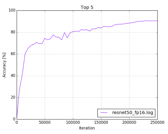
            caffe$ python plot_top5.py -s
models/resnet50/logs/resnet50_fp16.log
Your output should look similar to the following:
Figure 4. ResNet-50 FP16 training log
7.6.2. NVCaffe FP16 Example
For examples on optimization, refer to the models/resnet50/train_val_fp16.prototxt file.
After you have trained a neural network, you can optimize and deploy the model for GPU inferencing with TensorRT™ . For more information about optimizing and deploying using TensorRT, refer to the NVIDIA TensorRT documentation.
9.1. General FAQs
Q: What additional resources are available for how to use mixed precision?
A: Here are some additional resources that can help with understanding mixed precision:
- Mixed Precision Training (ICLR 2018).
- Mixed-Precision Training of Deep Neural Networks (NVIDIA Developer Blog).
Q: What is Automatic Mixed Precision (AMP) and how can it help with training my model?
A: Automatic Mixed Precision (AMP) makes all the required adjustments to train models using mixed precision, providing two benefits over manual operations:
- Developers need not modify network model code, reducing development and maintenance effort.
- Using AMP maintains forward and backward compatibility with all the APIs for defining and running models.
The benefits of mixed precision training are:
- Speed up of math-intensive operations, such as linear and convolution layers, by using Tensor Cores.
- Speed up memory-limited operations by accessing half the bytes compared to single-precision.
- Reduction of memory requirements for training models, enabling larger models or larger minibatches.
For more information, refer to Automatic Mixed Precision for Deep Learning.
Q: How does AMP automate mixed precision?
A: Using mixed precision training requires two steps:
- Porting the model to use the FP16 data type where appropriate.
- Using loss scaling to preserve small gradient values.
AMP automates both these steps. In particular in TF-AMP, this is controlled by means of a single environment variable.
Q: How does dynamic scaling work?
A: Dynamic loss scaling basically attempts to ride the edge of the highest loss scale it can use without causing gradient overflow, to make full use of the FP16 dynamic range.
It does so by beginning with a high loss scale value (say, 2^24), then in each iteration, checking the gradients for overflows (infs/NaNs). If none of the gradients overflowed, gradients are unscaled (in FP32) and optimizer.step() is applied as usual. If an overflow was detected, optimizer.step is patched to skip the actual weight update (so that the inf/NaN gradients do not pollute the weights) and the loss scale is reduced by some factor F (F=2 by default). This takes care of reducing the loss scale to a range where overflows are not produced. However, it's only half the story.
What if, at some later point, training has stabilized and a higher loss scale is permissible? For example, later in training, gradient magnitudes tend to be smaller, and may require a higher loss scale to prevent underflow. Therefore, dynamic loss scaling also attempts to increase the loss scale by a factor of F every N iterations (N=2000 by default). If increasing the loss scale causes an overflow once more, the step is skipped and the loss scale is reduced back to the pre-increase value as usual. In this way, by: reducing the loss scale whenever a gradient overflow is encountered, and Intermittently attempting to increase the loss scale, the goal of riding the edge of the highest loss scale that can be used without causing overflow is (roughly) accomplished.
Q: How do you increase the batch size when AMP is enabled? Do you just increase the batch size by 2?
A: It depends on how much memory you saved, which depends on the model. A quick way is to watch -n 0.5 nvidia-smi from a separate terminal while you launch your run, to see how much device memory you're using. In general, using a larger batch per GPU tends to improve utilization, as long as you obey the guidelines to allow Tensor Core usage (refer to Issue #221 for more information).
Q: How is AllowList/DenyList/InferList determined? What are the corresponding ops that are in each list?
A: We determine these based on our experience with numeric stability from our research. AllowList operations are operations that take advantage of our GPU Tensor Cores. DenyList operations are operations that may overflow the range of FP16, or require the higher precision of FP32. InferList operations are operations that are safely done in either FP32 or FP16. Typical ops included in each list are:
- AllowList: Convolutions, Fully-connected layers
- DenyList: Large reductions, Cross entropy loss, L1 Loss, Exponential
- InferList: Element-wise operations (add, multiply by a constant)
To view/review, modify, and recompile to experiment, or to use environment variables in our container to modify AllowList/DenyList, see:
- For TensorFlow, to modify, use this.
- For PyTorch, to modify, use this. Reinstall APEX, however, you don’t need to recompile PyTorch at this time.
Q: What are the minimum hardware and software requirements to use AMP?
A: In order to run AMP effectively, you need Tensor Cores in your GPU; for training, we recommend V100; and for inference, we recommend T4. You can access this hardware through cloud service providers (AWS, Azure or Google Cloud).
When using a framework, TensorFlow 1.14 supports AMP natively or support for AMP is available using NVIDIA’s containers 19.07+. In PyTorch, 1.0 AMP is available through APEX.
Q: How do I enable AMP for my deep learning training?
A: Enabling AMP is framework dependent:
- In TensorFlow, AMP is controlled by wrapping the optimizer as follows:
tf.train.experimental.enable_mixed_precision_graph_rewrite(opt)
- In PyTorch, AMP is available through the APEX extension:
            model, optimizer = amp.initialize(model, optimizer, opt_level="O1")
with amp.scale_loss(loss, optimizer) as scaled_loss:
    scaled_loss.backward()
- In MXNET, AMP is available through the contrib library:
            amp.init()
amp.init_trainer(trainer)
with amp.scale_loss(loss, trainer) as scaled_loss:
   autograd.backward(scaled_loss)
Q: What are the models that are suitable for AMP? And what kind of speed-up can I expect?
A: All models are suitable for AMP, although the speed-up may vary from model to model. The following table provides some examples of the speed-up for different models:
| Model Script | Framework | Data Set | FP32 Accuracy | Mixed Precision Accuracy | FP32 Throughput | Mixed Precision Throughput | Speed-up |
|---|---|---|---|---|---|---|---|
| BERT Q&A | TensorFlow | SQuAD | 90.83 Top 1% |
90.99 Top 1% |
66.65 sentences/sec | 129.16 sentences/sec | 1.94 |
| SSD w/RN50 | TensorFlow | COCO 2017 | 0.268 mAP |
0.269 mAP |
569 images/sec | 752 images/sec | 1.32 |
| GNMT | PyTorch | WMT16 English to German | 24.16 BLEU |
24.22 BLEU |
314,831 tokens/sec | 738,521 tokens/sec | 2.35 |
| Neural Collaborative Filter | PyTorch | MovieLens 20M | 0.959 HR |
0.960 HR |
55,004,590 samples/sec | 99,332,230 samples/sec | 1.81 |
| U-Net Industrial | TensorFlow | DAGM 2007 | 0.965-0.988 | 0.960-0.988 | 445 images/sec | 491 images/sec | 1.10 |
| ResNet-50 v1.5 | MXNet | ImageNet | 76.67 Top 1% |
76.49 Top 1% |
2,957 images/sec | 10,263 images/sec | 3.47 |
| Tacotron 2 / WaveGlow 1.0 | PyTorch | LJ Speech Dataset | 0.3629/-6.1087 | 0.3645/-6.0258 | 10,843 tok/s 257,687 smp/s |
12,742 tok/s 500,375 smp/s |
1.18/1.94 |
Values are measured with the model running on DGX-1V 8GPU 16G, DGX-1V 8GPU 32G, or DGX-2V 16GPU 32G.
When enabling AMP, there are other aspects to consider such as the reduction in memory and in bandwidth needed to train the mixed precision model.
Q: How much faster will my model run with AMP?
A: There are no precise rules for mixed precision speedups, but here are a few guidelines:
- The more time is spent in matrix multiplication (linear layers) or convolutions, the more Tensor Cores can accelerate the model. This means that "bigger" models often see larger speedups.
- In particular, very small linear and convolution layers will see limited benefit from AMP, since there is not enough math to fully exploit Tensor Cores.
- Mixed precision models use less memory than FP32, so it is possible to increase the batch size when running with AMP. Therefore, you can often increase the speedup by increasing the batch size after enabling AMP.
Q: How do I see reduced memory consumption?
A: In TensorFlow, set the allow_growth flag so it only allocates what it needs and view in nvidia-smi. For PyTorch, nvidia-smi can show memory utilization. The best way to test, is to try a larger batch size that would have otherwise led to out-of-memory when AMP is not enabled.
Q: What if I have already implemented manual mixed precision, how will AMP further improve my model performance? What benefits should I expect from AMP?
A: If the code is already written in such a way to follow the NVIDIA Mixed Precision Training Guide, then AMP will leave things as they are.
Q: Why do I observe only a little speedup with AMP turned on?
A: First, you need to identify the bottleneck in your workflow, is it data I/O or compute bound? To find out what is limiting the performance of your workflow use DLProf to profile it.
If the slowest part of the workflow is in the GPU, check if the layers of your model are actually making use of mixed precision. This can be done in a TensorBoard extension after profiling your network with DLProf, or manually by profiling with Nsight Systems or nvprof and looking for kernel names including the strings [i|s|h]884 or [i|s|h]1688 (for example, volta_h884gemm_… or turing_fp16_s1688cudnn_fp16_…).
Some layers of a network are DenyListed, meaning that they cannot use mixed precision for accuracy reasons. The DenyList is framework dependent. Refer to the following resources for more information:
Furthermore, Tensor Cores are optimizing GEMMs (generalized (dense) matrix-matrix multiplies) operations, there are restrictions on the dimensions of the matrices in order to effectively optimize such operations:
- For A x B where A has size (M, K) and B has size (K, N):
- N, M, K should be multiples of 8
- GEMMs in fully connected layers:
- Batch size, input features, output features should be multiples of 8
- GEMMs in RNNs:
- Batch size, hidden size, embedding size, and dictionary size should be multiples of 8
Q: Is accuracy worse when AMP is turned on?
A: AMP is designed to leave accuracy unchanged with respect to FP32 training. And, in practice, we never observed noticeable degradation of accuracy when training with AMP.
Q: What if the model code crashes after I have enabled AMP?
A: First, make sure that your model doesn’t crash without using AMP. Then, if you have experienced such issues after enabling AMP, file a bug.
Q: How do I know that AMP is working for me or Tensor Cores are being enabled?
A: The log outputs whether AMP is working, and is framework specific. In TensorFlow, for instance, you will see log messages similar to the following:
            TF AMP log messages are of the form ‘Converted 405/4897 nodes to float16 precision using
        2 cast(s) to float16 (excluding Const and Variable casts)
9.2. TensorFlow FAQs
Q: Is Automatic Mixed Precision (AMP) dependent on a TensorFlow version or can any TensorFlow version enable AMP?
A: AMP is available in the NGC TensorFlow containers starting from 19.03 and is enabled using the TF_ENABLE_AUTO_MIXED_PRECISION=1 environment variable. It is now enabled by wrapping the optimizer object as follows:
opt = tf.train.experimental.enable_mixed_precision_graph_rewrite(opt)
More information is available in the following webinar. Starting with TensorFlow 1.14, AMP will be available natively in the framework.
Q: What is the scheme for TensorFlow to decide which operations to cast to FP16 (which level of the graph or where to decide)? Does TensorFlow also keep a DenyList and an AllowList like PyTorch?
A: Our GTC Silicon Valley session S91029, Automated Mixed-Precision Tools for TensorFlow Training discusses how this works. TensorFlow also uses the DenyList and AllowList concepts, but with some subtle differences because TensorFlow has the advantage of a static graph to analyze and convert.
Q: What is TF-AMP and what is the goal?
A:The top-level goal is that our customers who use TensorFlow to train on V100 have a great mixed precision training experience utilizing all the acceleration possible offered by the hardware. That means accuracy that matches FP32 and real speedups without much manual effort. In practice, achieving that goal requires a few things to happen:
- Correctly porting the model to mixed precision. Meaning, updating
dtypesin code to FP16 as well as making sure that numerically “unsafe” operations stay in FP32. - Using loss scaling to avoid gradient flush-to-zero (important for accuracy).
- The existence of fast FP16 kernels for the relevant operations, along with the software stack from the user down to the kernels ensuring that those kernels get called correctly.
Q: How is TF-AMP implemented?
A:TF-AMP optimizes the model graph mainly by:
- Inserting the appropriate cast operations into your TensorFlow graph to use FP16 execution and storage where appropriate; this enables both the use of Tensor Cores along with memory storage and bandwidth savings.
- Turn on automatic loss scaling inside the Optimizer object.
It is possible to separately enable the automatic insertion of cast operations and automatic loss scaling. For more details, refer to this NVIDIA TensorFlow User Guide.
It must be emphasized that this is only one part of making mixed precision successful, the most important part is to ensure that these changes do not reduce accuracy.
Q: Is AMP dependent on a TensorFlow version or can any TensorFlow version enable AMP?
A: AMP is available in the NGC TensorFlow containers:
- The environment variable method for enabling TF-AMP is available starting in 19.03.
- The optimizer-wrapper method for enabling TF-AMP is available starting in the 19.06 container.
Furthermore AMP is available with the official distribution of TensorFlow starting with version 1.14. More information is available in the following webinar.
Q: How does AMP know which layer of the model to optimize?
A: AMP maintains lists of the layers that can be optimized:
- AllowList: cast everything to FP16
- DenyList: cast everything to FP32
- Everything else: cast everything to match the widest input type (can’t allow type mismatch)
The TensorFlow list is located here. TensorFlow has the advantage of a static graph to analyze and convert with respect to other frameworks.
Our GTC Silicon Valley session S91029, Automated Mixed-Precision Tools for TensorFlow Training discusses how this works in more detail.
Q: How can I see what changes automatic mixed precision makes to my model?
A: Because automatic mixed precision operates at the level of TensorFlow graphs, it can be challenging to quickly grasp the changes it makes: often it will tweak thousands of TensorFlow operations, but those correspond to many fewer logical layers. You can set the environment variable TF_CPP_VMODULE="auto_mixed_precision=2" to see a full log of the decisions automatic mixed precision makes (note that this may generate a lot of output).
Q: Why do I see only FP32 datatypes in my saved model GraphDef?
A: When you save a model graph or inspect the graph with Session.graph for Session.graph_def, TensorFlow returns the unoptimized version of the graph. TF-AMP works as an optimization pass over the original graph, so its changes are not included in the unoptimized graph. You can set the environment variable TF_AMP_LOG_PATH=some_directory, and TF-AMP will save pre- and post-optimization copies of each graph it processes to that directory.
There will be many hard-to-distinguish graph files since TensorFlow processes initialization (for example) as a disjoint graph.
Q: Why do I see
step=0
repeated multiple times when training with TF-AMP?
A: The automatic loss scaling algorithm that TF-AMP enables can choose to “skip” training iterations as it searches for the optimal loss scale. When it does so, it does not increment the global step count. Since most of the skips occur at the beginning of training (usually fewer than ten iterations), this behavior manifests as multiple iterations where the step counter stays at zero.
Q: How are user-defined custom TF operations handled?
A: By default, TF-AMP will leave alone any op types it doesn’t know about, including custom operations. That means the types of op’s inputs and outputs are not changed, and TF-AMP will insert casts as necessary to interoperate with the rest of the (possibly-changed) graph. If you would like to make TF-AMP aware of a custom op type, there are three environment variables you can use:
-
TF_AMP_ALLOWLIST_ADD - These are ops for which it is worth casting the inputs to FP16 to get FP16 execution. Mostly, they are ops that can take advantage of Tensor Cores.
-
TF_AMP_INFERLIST_ADD - These are ops for which FP16 execution is available, so they can use FP16 if the inputs happen to already be in FP16 because of an upstream AllowList op.
-
TF_AMP_DENYLIST_ADD - These are ops for which FP32 is necessary for numerical precision, and the outputs are not safe to cast back to FP16. Example ops include Exp and Log.
Each of these environment variables takes a comma-separated list of string op names. For example, you might set export TF_AMP_ALLOWLIST_ADD=MyOp1,MyOp2. The op name is the string name used in the call to REGISTER_OP, which corresponds to the name attribute on the operation’s OpDef.
Q: Can I change the algorithmic behavior of automatic mixed precision?
A: The primary lever for controlling automatic mixed precision behavior is to manipulate what ops lie on each of the AllowList, InferList, and DenyList. You can add ops to each using the three environment variables above, and there is a corresponding variable TF_AUTO_MIXED_PRECISION_GRAPH_REWRITE_{ALLOWLIST,INFERLIST,DENYLIST}_REMOVE to take built-in ops off of each list.
Q: Why doesn’t my model achieve full accuracy when I enable AMP?
A: The most likely explanation is that loss scaling is not being applied during gradient evaluation. This can happen if the optimizer is not wrapped by tf.trian.experimental.enable_mixed_precision_graph_rewrite() or if gradients are computed directly using tf.gradients() rather than with Optimizer.minimize() or Optimizer.compute_gradients().
Q: Do we have examples or documentation showing how to use AMP with tf.gradients() along with static and/or dynamic loss scaling?
A: For static loss scaling, it’s straightforward:
            loss = some_loss()
loss *= loss_scale # Scale by the loss scale
scaled_grads = tf.gradients(loss, …) # Compute gradients

# Now unscale, handling sparse grads
grads = []
for scaled_grad in scaled_grads:
  if scaled_grad is not None:
    if isinstance(scaled_grad, tf.IndexedSlices):
      grads.append(tf.IndexedSlices(
                    scaled_grad.values * (1. / loss_scale),
                    scaled_grad.indices,
                    scaled_grad.dense_shape))
    else:
      grads.append(scaled_grad * (1. / loss_scale))
  else:
    grads.append(None)

# Now use `grads` as you would normally
9.3. PyTorch FAQs
Q: Is Automatic Mixed Precision (AMP) dependent on a PyTorch version or can any PyTorch version enable AMP?
A: AMP with CUDA and CPP extensions requires PyTorch 1.0 or later. The Python-only build might be able to work with PyTorch 0.4, however, 1.0+ is strongly recommended.
Q: How does dynamic scaling choose a good scaling factor?
A: Dynamic loss scaling basically attempts to ride the edge of the highest loss scale it can use without causing gradient overflow, to make full use of the FP16 dynamic range.
It does so by beginning with a high loss scale value (say, 2^24), then in each iteration, checking the gradients for overflows (infs/NaNs). If none of the gradients overflowed, gradients are unscaled (in FP32) and optimizer.step() is applied as usual. If an overflow was detected, optimizer.step is patched to skip the actual weight update (so that the inf/NaN gradients do not pollute the weights) and the loss scale is reduced by some factor F (F=2 by default). This takes care of reducing the loss scale to a range where overflows are not produced. However, it's only half the story. What if, at some later point, training has stabilized and a higher loss scale is permissible? For example, later in training, gradient magnitudes tend to be smaller, and may require a higher loss scale to prevent underflow. Therefore, dynamic loss scaling also attempts to increase the loss scale by a factor of F every N iterations (N=2000 by default). If increasing the loss scale causes an overflow once more, the step is skipped and the loss scale is reduced back to the pre-increase value as usual. In this way, by:
- Reducing the loss scale whenever a gradient overflow is encountered, and
- Intermittently attempting to increase the loss scale, the goal of riding the edge of the highest loss scale that can be used without causing overflow is (roughly) accomplished.
Q: How do you increase the batch size when AMP is enabled? Do you just increase the batch size by 8?
A: It depends on how much memory you saved, which depends on the model. A quick-and-dirty way is to watch -n 0.5 nvidia-smi from a separate terminal while you launch your run, to see how much device memory you're using. In general, using a larger batch per GPU tends to improve utilization, as long as you obey the guidelines to allow Tensor Core usage (refer to Issue #221 for more information).
Q:Is AMP dependent on a PyTorch version or can any PyTorch version enable AMP?
A: AMP with CUDA and CPP extensions requires PyTorch 1.0 or later. The Python-only build might be able to work with PyTorch 0.4, however, 1.0+ is strongly recommended.
Q: How to use O0, O1, O2, O3? Which is recommended for AMP? What are the differences?
- Use O0 for baseline FP32.
- Use O1 for AMP.
Note:
In the future, AMP O1 functionality will be moved upstream.
- O2 is slightly faster, but could be harder to converge/stabilize, or may not converge to FP32 results. In O2, all the ops are in FP16, so generally not recommended.
- Use O3 for everything in FP16, no primary weights. O3 is intended for performance comparison to see the AMP overhead.
Q: Can AMP save checkpoints of the model in FP32?
A: O1 checkpoints of the model will be saved in FP32, with O2 checkpoints of the model will not be saved in FP32, and the optimizer primary weights must be saved separately. The best practice is always to use O1 to save checkpoints.
9.4. MXNet FAQs
Q: Is Automatic Mixed Precision (AMP) dependent on an MXNet version or can any MXNet version enable AMP?
A: AMP is available in the NGC MXNet container starting from 19.04. Starting with MXNet 1.5, AMP will be available natively in the upstream framework.
Notice
This document is provided for information purposes only and shall not be regarded as a warranty of a certain functionality, condition, or quality of a product. NVIDIA Corporation (“NVIDIA”) makes no representations or warranties, expressed or implied, as to the accuracy or completeness of the information contained in this document and assumes no responsibility for any errors contained herein. NVIDIA shall have no liability for the consequences or use of such information or for any infringement of patents or other rights of third parties that may result from its use. This document is not a commitment to develop, release, or deliver any Material (defined below), code, or functionality.
NVIDIA reserves the right to make corrections, modifications, enhancements, improvements, and any other changes to this document, at any time without notice.
Customer should obtain the latest relevant information before placing orders and should verify that such information is current and complete.
NVIDIA products are sold subject to the NVIDIA standard terms and conditions of sale supplied at the time of order acknowledgement, unless otherwise agreed in an individual sales agreement signed by authorized representatives of NVIDIA and customer (“Terms of Sale”). NVIDIA hereby expressly objects to applying any customer general terms and conditions with regards to the purchase of the NVIDIA product referenced in this document. No contractual obligations are formed either directly or indirectly by this document.
NVIDIA products are not designed, authorized, or warranted to be suitable for use in medical, military, aircraft, space, or life support equipment, nor in applications where failure or malfunction of the NVIDIA product can reasonably be expected to result in personal injury, death, or property or environmental damage. NVIDIA accepts no liability for inclusion and/or use of NVIDIA products in such equipment or applications and therefore such inclusion and/or use is at customer’s own risk.
NVIDIA makes no representation or warranty that products based on this document will be suitable for any specified use. Testing of all parameters of each product is not necessarily performed by NVIDIA. It is customer’s sole responsibility to evaluate and determine the applicability of any information contained in this document, ensure the product is suitable and fit for the application planned by customer, and perform the necessary testing for the application in order to avoid a default of the application or the product. Weaknesses in customer’s product designs may affect the quality and reliability of the NVIDIA product and may result in additional or different conditions and/or requirements beyond those contained in this document. NVIDIA accepts no liability related to any default, damage, costs, or problem which may be based on or attributable to: (i) the use of the NVIDIA product in any manner that is contrary to this document or (ii) customer product designs.
No license, either expressed or implied, is granted under any NVIDIA patent right, copyright, or other NVIDIA intellectual property right under this document. Information published by NVIDIA regarding third-party products or services does not constitute a license from NVIDIA to use such products or services or a warranty or endorsement thereof. Use of such information may require a license from a third party under the patents or other intellectual property rights of the third party, or a license from NVIDIA under the patents or other intellectual property rights of NVIDIA.
Reproduction of information in this document is permissible only if approved in advance by NVIDIA in writing, reproduced without alteration and in full compliance with all applicable export laws and regulations, and accompanied by all associated conditions, limitations, and notices.
THIS DOCUMENT AND ALL NVIDIA DESIGN SPECIFICATIONS, REFERENCE BOARDS, FILES, DRAWINGS, DIAGNOSTICS, LISTS, AND OTHER DOCUMENTS (TOGETHER AND SEPARATELY, “MATERIALS”) ARE BEING PROVIDED “AS IS.” NVIDIA MAKES NO WARRANTIES, EXPRESSED, IMPLIED, STATUTORY, OR OTHERWISE WITH RESPECT TO THE MATERIALS, AND EXPRESSLY DISCLAIMS ALL IMPLIED WARRANTIES OF NONINFRINGEMENT, MERCHANTABILITY, AND FITNESS FOR A PARTICULAR PURPOSE. TO THE EXTENT NOT PROHIBITED BY LAW, IN NO EVENT WILL NVIDIA BE LIABLE FOR ANY DAMAGES, INCLUDING WITHOUT LIMITATION ANY DIRECT, INDIRECT, SPECIAL, INCIDENTAL, PUNITIVE, OR CONSEQUENTIAL DAMAGES, HOWEVER CAUSED AND REGARDLESS OF THE THEORY OF LIABILITY, ARISING OUT OF ANY USE OF THIS DOCUMENT, EVEN IF NVIDIA HAS BEEN ADVISED OF THE POSSIBILITY OF SUCH DAMAGES. Notwithstanding any damages that customer might incur for any reason whatsoever, NVIDIA’s aggregate and cumulative liability towards customer for the products described herein shall be limited in accordance with the Terms of Sale for the product.
Android, Android TV, Google Play and the Google Play logo are trademarks of Google, Inc.
Trademarks
NVIDIA, the NVIDIA logo, CUDA, Merlin, RAPIDS, Triton Inference Server, Turing and Volta are trademarks and/or registered trademarks of NVIDIA Corporation in the United States and other countries. Other company and product names may be trademarks of the respective companies with which they are associated.