Enterprise RAG Retrieval - Accuracy, Performance and Cost Efficiency

Retrieval-Augmented Generation (RAG) has emerged as a critical technology for enterprises looking to integrate their business data with AI inference capabilities. As organizations move from experimental AI chatbots to production-scale deployments, the complexity of building and scaling a robust, scalable AI factory for RAG becomes apparent. This document highlights best practices for scaling and sizing enterprise-ready RAG inference solutions.

RAG Enterprise Challenge

Enterprises need AI inference with RAG to scale to thousands of concurrent users, ingest millions of documents, while generating accurate and context-relevant responses to queries.

To build an AI factory for RAG, enterprises must be able to size and scale their infrastructure for the inference use cases they are looking to deploy.

An enterprise is deploying RAG AI inference solutions and needs answers to these questions:

• An IT customer service chatbot for 25 concurrent users; what is the minimum deployment needed? How many nodes and GPUs are required?

• A large scale RAG deployment for 200 concurrent users servicing multiple RAG use cases; IT service chatbot, code generation, meeting recap, deep research; what is the recommended initial deployment size? How does it scale to include more use cases and more users?

Build a scalable AI factory for RAG

To effectively scale the AI factory for RAG, it must have a pluggable microservice architecture with predictable linear scaling.

For sizing an AI Factory for RAG; there needs to be clearly defined use cases and benchmarking methodology with tools to evaluate the accuracy and performance to meet the required SLAs for data ingestion rate and user request rate.

The focus for this guide is to provide best practices for achieving high RAG retrieval performance and accuracy. It also provides scaling guidelines for individual RAG services while maintaining latency thresholds for RAG use cases Chat vs Summarization. At the same time the guide looks to maintain cost efficiencies with predictable linear scaling and provide high performance per $ (TCO cost).

RAG Retrieval workflow

The RAG server is the data orchestrator sending requests and processing responses to and from other services in the retrieval pipeline.

It is responsible for receiving user queries and then initiating calls to Nemotron embed model, Milvus Vector database (VDB), Nemotron rerank model, NIM LLM and NeMo Evaluator (AI Agent) or other third party microservices in the retrieval pipeline. Finally, the RAG server is responsible for sending the final response to the user query.

1. User sends the request Query (ISL) to RAG Server

2. RAG server sends tokenized Query to Embedding NIM to create an embedding vector

3. Next the embedding vector is sent to Milvus VDB to perform an Approximate Nearest Neighbor (ANN) search to return the VDB top-k (say 10) data chunks that are relevant to the Query embedding vector.

4. Then Nemotron reranking model ranks and filters chunks to return Reranker TopK (say 4) data chunks that are most relevant as context for the Query.

5. The RAG server then sends the original User Query + Context (4 data chunks received from the Reranker) + System Prompt to the NIM LLM as context for response generation.

6. Finally the RAG server forwards the NIM LLM Response (OSL) to the user.

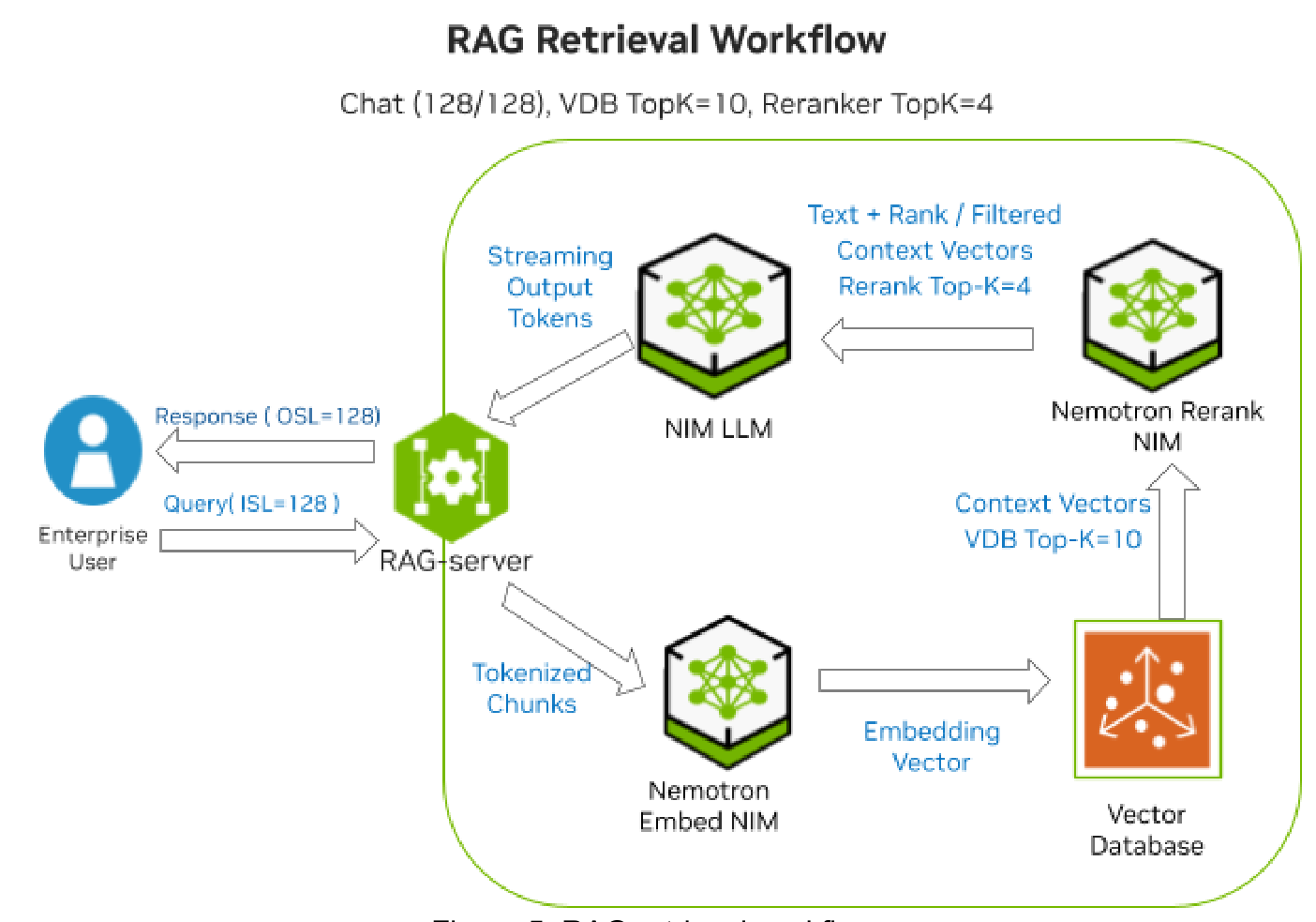
Figure 1 RAG retrieval workflow

Key Metrics for RAG Retrieval

Metrics are crucial and required to measure success when deploying and scaling RAG; to validate the performance and accuracy. For a RAG AI inference use case the key parameters and metrics are defined in the table below.

Metric or Parameter	Description
ISL/OSL	Input and output characteristics defined by input sequence length (ISL) which is the user prompt or query length in tokens and expected output sequence length (OSL) in tokens. With RAG the ISL gets padded with additional Context retrieved from the vector DB and the System Prompt providing instructions to LLM to only use the provided context to answer the user query.
Concurrent requests (CR)	Concurrency (CR) defines the number of active in-flight user requests being served by the RAG retrieval pipeline. It is a measure of peak usage at given Latency. It defines the load when benchmarking the RAG retrieval pipeline.
Latency metrics	The Latency metrics TTFT, ITL, E2E Request Latency are used to define Latency SLAs for use cases. Time to First Token (TTFT) - is the time taken to receive the first response token from the RAG service after sending the user query. It is an indication of user responsiveness. It is also referred to as the Prefill Latency. The RAG pipeline primarily impacts TTFT due to additional overhead from retrieved context that significantly increases the input sequence length (ISL). The amount of context depends on the Chunk Size, the number of chunks (TopK) retrieved from the vector DB and filtered by the reranker. RAG ISL = User-Query + VDB Context + System-Prompt = User-Query + [ TopK X Chunk-Size] + System-Prompt. Inter Token Latency (ITL) - is the average time between tokens. It is responsible for the Decode Latency and Generation time. The RAG retrieval pipeline does not affect ITL as much so it remains fairly close to what is expected when querying LLM directly. Inter-token latency (ITL) rises with longer ISL, since each new token must attend across a larger KV cache. However, the impact on ITL is subtler and sublinear compared to the sharp increase in first-token latency. Modern attention kernels (e.g., FlashAttention, paged KV) reduce the growth curve, but they do not eliminate it. E2E request Latency - includes the time to first token (TTFT) and the total token Generation time. The generation time depends on inter-token latency (ITL) and expected size of OSL. Summarization, Report Generation and Research/Analysis use cases have larger OSL.
Throughput metrics	The output throughput metrics tokens per second (TPS) and requests per second (RPS) measure the overall performance of the RAG retrieval service across all requests. Tokens per second (TPS) is output tokens generated per second by the RAG service across all user requests being processed. Requests per second (RPS) - output throughput can also be measured as requests per second. It is the number of RAG retrieval requests that are being processed per second. Per user throughput (TPS) - is the output tokens generated per second per user. It is measured in Tokens per second (TPS). It is a measure of User responsiveness (per user latency) or overall user experience (UX). As the number of concurrent requests (active users) increases, the Per user throughput decreases. Typically at maximum output throughput (highest TPS), the Per user throughput is poor. For Balanced Performance, maximize Output Throughput (TPS) X Per User Throughput (TPS).
Performance per $ (TCO)	Performance per Total Cost of Ownership (TCO) dollar, or performance-per-$ measures the RAG retrieval compute (CPU/GPU) efficiency, or throughput achieved relative to the full investment cost. The RAG Retrieval TCO is measured in terms of GPU Cost to generate 1 Million tokens.

\[\text{Cost per Million tokens (\$)} = \frac{\text{Retrieval GPUs} \times \text{GPU hourly cost}}{\text{Output Throughput (TPS)} \times 3600} \times 1{,}000{,}000\]

Table 1. RAG metrics and parameters

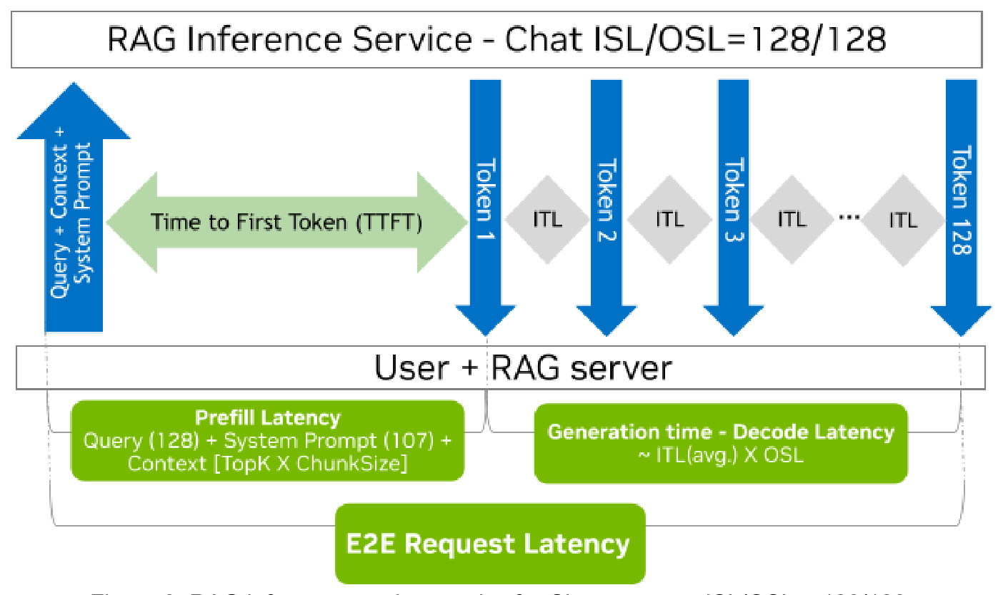
Figure 2 RAG inference service metrics for Chat use case ISL/OSL = 128/128

Let’s review some RAG specific parameters:

RAG parameters	Description
Chunk Size (defined during ingestion, cannot be changed after)	Chunking is performed during initial data extraction and preprocessing phase of ingestion; where documents are split into fixed-size token chunks that can be efficiently embedded, indexed, retrieved, and used as context during response generation.
Top-K (the k in top-k is user configurable and defined during retrieval)	Top-K is the top-ranked, relevant text chunks retrieved and included with context sent to the LLM for response generation. VDB Top-K is the number of chunks retrieved from the vector DB. If the reranker is enabled then the Reranker Top-K defines the number of filtered chunks sent to the LLM as context.

Table 2. RAG specific parameters

Target Use cases

The first step to benchmarking AI Inference use cases is to define load/performance requirements and metrics to measure. Let’s look at RAG Chat use case for Enterprise and flush out the requirements; ISL/OSL, peak usage (concurrent requests CR), Latency SLAs and data ingestion as shown below.

Usecase	Enterprise Requirements
Chat	ISL/OSL: 128/128 TTFT p90: 3s-5s e2e_latency p90: 5s-10s Org size: 1000 Concurrency: 20% Concurrent request: 200 Request rate: 40 RPS Data: 30% multimodal, 70% text Type: PDF, MD, Excel, S3 parquet ingest: on-demand or off-peak (bulk) Size: 5MB Ingest rate: 1K-3K docs/hour IT or customer service chat: Short query short response; single-turn conversations. Input/Output: short ISL(128 tokens) and short OSL(128 tokens). SLA: Low Latency; High Concurrency; High accuracy and concise response (one shot, no thinking). AI Chat use case requires low Latency and support for high request rate (requests per second). It is also critical that responses are concise, relevant, accurate and grounded based on the context provided. Required first response in under 3s-5s; Use the 90th percentile TTFT p90 ≤ 3-5s; Required End-to-end response in 5s-10s: e2e request latency ≤ 5-10s. Assuming Concurrency (CR) of 20% for organization size of 1000, Peak usage: 200 concurrent requests with sustained request rate of 40 requests per second (RPS). data: product guides, blogs, bug reports; file type: MD, PDF, PPT, WORD, EXCEL, S3 parquet; Data Modality: 70% Text-only, 5% images, 10% charts, 15% tables. Ingestion: on-demand using Drag and Drop or Bulk ingest data during off-peak hours. Size: 10-20 GB per day; recommended ingest rate 1GB/hr
Summarization/Analysis	ISL/OSL: 1024/512 TTFT: 10-15s e2e_latency: 30s Org size: 1000 Concurrency: 10% Concurrent request: 100 Request rate: 6 RPS Data: 80% text; 20% multimodal Type: Email, Meeting notes, PDF, MD, PPT Bulk Ingest: continuous or off-peak Size: 50-100 MB; Ingest rate: 3-5K docs/hour Document summarization, meeting recap, research report review, multi-turn conversation. For summarization with multiturn conversations: ISL includes history of previous conversations. Input/Output: Long ISL (1024 tokens); Medium OSL (512 tokens). SLA: Medium Latency; Medium Concurrency; end-to-end response latency needs to be reasonable; High accuracy and brief summary response (one-shot); some user interactivity with thinking enabled. For summarization, initial brief thinking tokens to show responsiveness while large context is being processed; Reasonable latency in initial response time followed by accurate, grounded and brief summary response. Fast ingestion rate for multi-modal documents; and accuracy and relevance of response are critical. Average first response in under 10s; excluding thinking tokens; Average TTFT ≤ 10-15s. Average e2e request latency ≤ 30s (each turn). Total request latency ≤ 60s-120s (over multiple turns). Assuming Concurrency (CR) of 10% for organization size of 1000, Peak usage: 100 concurrent requests with sustained request rate of 6 requests per second (RPS). data: emails, meeting transcripts, documents, presentations, research papers. File type: PDF, MD, PPT, DOC; Data modality: 80% text, 5% images, 5% charts, 10% tables. data ingestion: continuous from repo or off-peak using bulk ingest. Size: 50-100MB; required ingest rate: 3-5K docs/hour
Generation	ISL/OSL: 128/2048 TTFT p90: 6-10s e2e_latency: 60-120s Concurrency: 5% Concurrent request: 50 Org size: 1000 Request rate: 2 RPS Data: 90% text; 10% multimodal Type: code (python, bash, json, yaml), research papers (MD, PDF) Bulk Ingest: continuous or off-peak Size: 100-200 MB; Ingest rate: 10K docs/hour, 10 MB/s Code generation, analysis, debugging; problem solving, chain of thought reasoning; multi-step agentic workflows, research report creation, analyze data, create charts. Input/Output: Short ISL(128) and Long OSL (2048). Faster initial response but end-to-end response time dominated by long OSL and reasoning and thinking enabled. SLA: High Latency; Medium Concurrency; High Accuracy. High user interactivity with thinking and reasoning enabled; deep reasoning and multi step planning. Early responses are required to show logical thinking and planning next steps; however end-to-end request latency is not as critical as long as progress is being made towards addressing the issue. Interactivity and user response time are important. Both first response and E2E Response Latency need to be reasonable; code review, root cause analysis and efficient code generation is critical. Required first response in under 6s; excluding thinking tokens; Average TTFT ≤ 6s; 90th percentile TTFT ≤ 10s. Average e2e request latency ≤ 60-120s. Assuming Concurrency (CR) of 5% for organization size of 1000, Peak usage: 50 concurrent requests with sustained request rate of 2 requests per second (RPS). Data: code, scripts, config files in repo, research papers. File type: code, scripts, raw data, python(.py), bash (.sh), json, research papers (PDF, MD, DOC). Data modality: 90% text, 8% tables, 3% charts. data ingestion: on the fly continuous data ingest from repo. Size: 100 MB. Required ingest rate: 10K docs/hour or 10MB/s

Table 3. Enterprise RAG use case requirements

RAG Balanced Performance

Scaling RAG inference requires balancing Concurrency and Latency; driving high output throughput while still maintaining user responsiveness.

For the RAG pipeline, Optimal or Balanced Performance occurs when optimizing both Output Throughput and User responsiveness (Per User Throughput). This typically occurs at the knee of the graph when plotting Output Throughput against Per User Throughput (highlighted in green); in this region Output Throughput(TPS) X User Throughput(TPS) is the maximum.

Most RAG use cases that don’t require very strict latency constraints but still require reasonable user responsiveness and can operate in the Balanced Performance or green region.

Balanced Performance balances output throughput, user responsiveness and performance per $ (TCO cost) and drives overall revenue of the AI inference application.

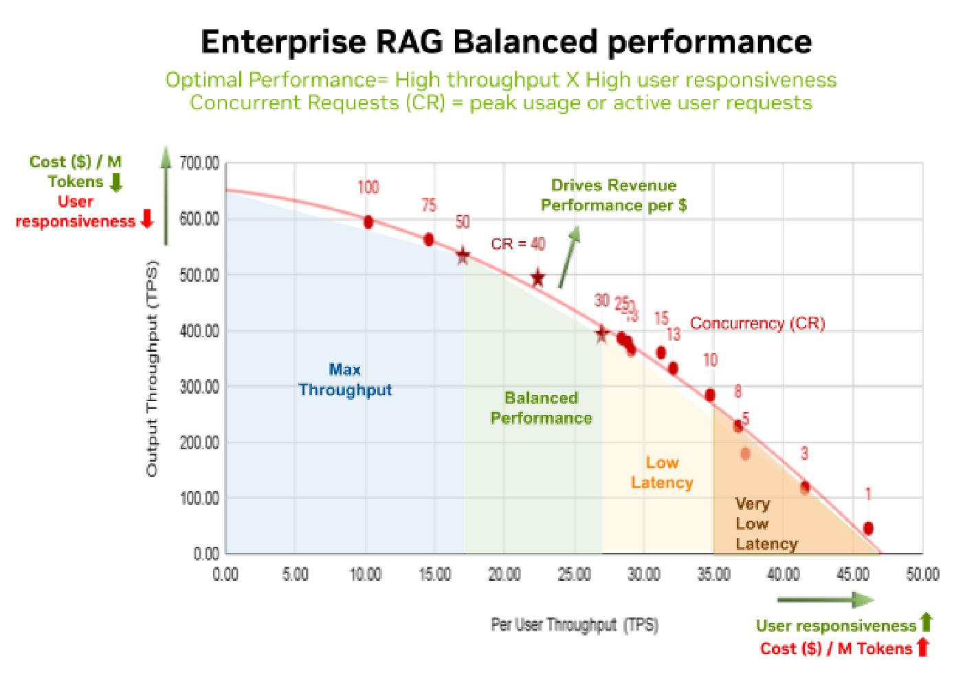
Figure 3 Enterprise RAG with Balanced Performance

Understanding Balanced performance

For AI Inference performance, balance application performance against per user performance measured as Output Throughput (TPS) vs Per User Throughput(TPS), where output throughput drives revenue (Cost($) per Million tokens) and User Throughput defines User responsiveness or User experience (per user latency). When the RAG service throughput is increased by increasing the number of Peak users or Concurrent Requests; the latency for each individual user also increases resulting in reduced per user throughput (TPS) and worse user experience (poor user responsiveness). Per User throughput is output tokens per second for one user. The right balance between Output Throughput (TPS) and Per User Throughput (TPS) is found by plotting the graph below for different Concurrent Requests (increment CR from 1 to 100).

Balanced Performance occurs when optimizing both Output Throughput and User responsiveness (Per User Throughput). This typically occurs at the knee of the graph when plotting Output Throughput against Per User Throughput (highlighted in green); in this region Output Throughput X User Throughput is the maximum.

In the sample chart below, Balanced Performance occurs at Concurrency = 40, and the range (green region) selected for Balanced Performance is with Peak Users CR=30-50. Select a smaller or wider range around this point CR=40 to be the Balanced Performance range for the Enterprise RAG service.

It is recommended to operate the Enterprise RAG service so that performance remains in the Balanced Performance or green region. Balanced Performance ensures best performance per $ (cost) and drives overall revenue of the AI inference application. Taking the sample chart above, for Balanced Performance, operate the RAG service with Peak Users or Active users between 30 and 50.

Moving to the left on the X-axis of the graph (highlighted in blue), the Output Throughput increases until it saturates, Max. Throughput region. In this region the User responsiveness decreases significantly. This region supports more Peak users or Concurrent Requests (CR) but per user latency is high. Each user needs to wait much longer to get a response.

Moving to the right on the X-axis of the graph (highlighted in yellow and orange) these are the Low Latency (and Very Low Latency) regions. In these regions User responsiveness or Per User Throughput increases, however the Output Throughput drops and Cost ($) per Million tokens decreases. This region is recommended for use cases where low latency is critical e.g. Customer Service AI chatbot. This region supports fewer Peak users or Concurrent Requests (CR) but User responsiveness is increased significantly.

Key Benchmarks for RAG Retrieval

Define the State of Art (SOTA) or Speed of Light (SOL) benchmark to compare against to validate the Enterprise RAG performance.

For Enterprise RAG Retrieval, there are 3 benchmarks that will be tracked for each use case:

• RAG-ON - RAG Retrieval pipeline with overhead from all components (Embedding NIM, Retrieval from Milvus VDB, Reranking NIM)

• RAG-OFF - standard inference with original User Query ISL sent directly to LLM.

• RAG-OFF with RAG ISL (SOL) - Simulated RAG inference with RAG ISL (User Query

  • Context + System Prompt) sent directly to LLM.

Benchmark overview

Consider an example for First Token Latency or Time to first Token chart for Chat 128/128 use case with VDB TopK=4 (4 chunks being retrieved from VDB and sent to LLM) and Chunk Size 256 tokens (average Chunk Size 243 tokens) with all 3 benchmarks as shown below.

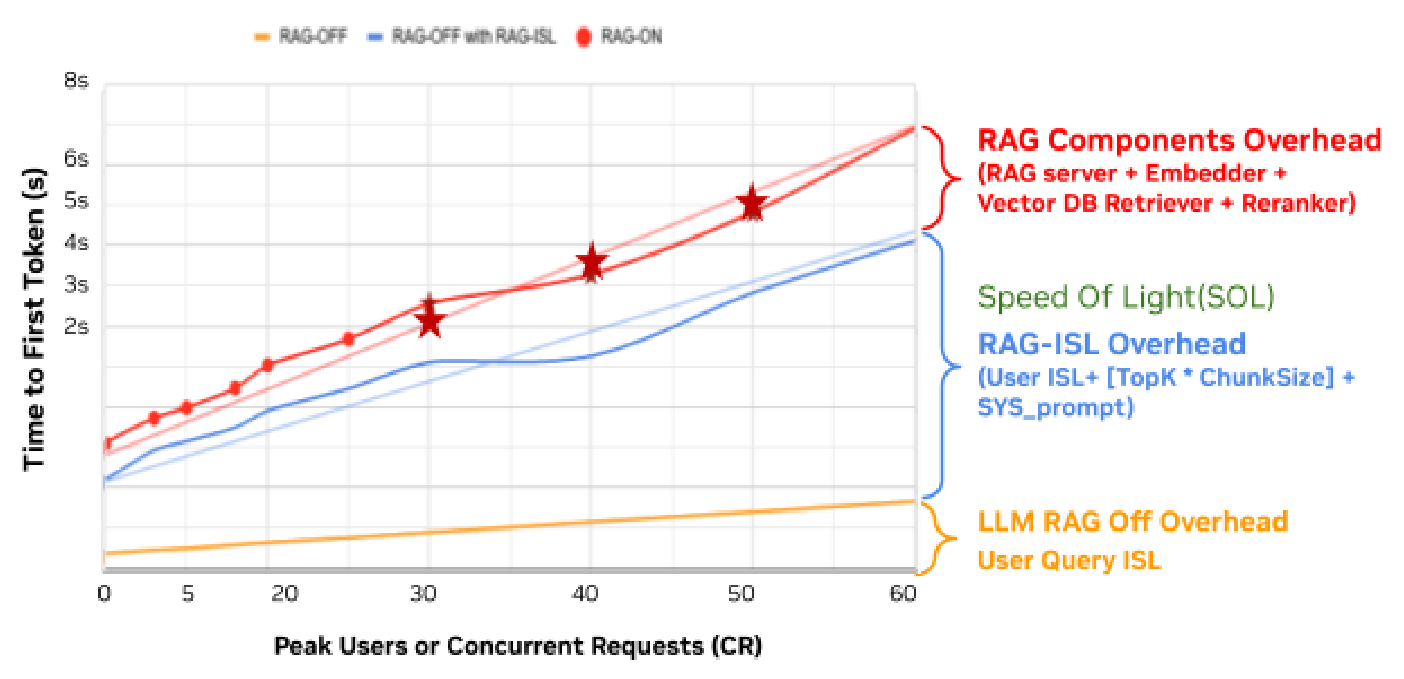
Figure 4 Benchmark Overview: TTFT Latency Comparison - RAG-ON vs RAG-OFF with RAG-ISL (SOL) vs RAG-OFF

The RAG-OFF (yellow) latency line has the least overhead. It shows the impact of the User Query ISL. This impact can be reduced by scaling the LLM or changing the Model (Size, precision, profile) or using next generation GPU.

The SOL benchmark RAG-OFF with RAG-ISL (blue) latency line best simulates RAG (without the actual components). It shows significant overhead on top of the RAG-OFF (yellow) line. This indicates the impact of the added Context (4 Chunks X 243 Avg.Chunk Size). The larger the chunk size selected and the more the number of VDB chunks sent to the LLM the larger the latency overhead. To reduce this impact, it is crucial to select the Chunk size and the TopK appropriately to ensure good performance and accuracy.

The RAG-ON (red) latency line shows additional overhead on top of the RAG-OFF with RAG-ISL (blue) line. This shows the impact of the latency from RAG retrieval components(RAG server, Embedding NIM, Retriever, Milvus VDB, Reranker). This overhead can only be reduced by adding more resources or scaling the individual components as the users or concurrent requests increase.

Deep Dive on Benchmark measurement

Benchmark	Endpoint	Chat ISL	Description
RAG-ON	RAG Server	User Query ISL. For Chat, ISL => 128 tokens. RAG ISL = User Query + Context + SYS Prompt. RAG ISL = User Query + [TopK * CHUNK_SIZE] + SYS PROMPT_SIZE	User query (prompt) is sent to the RAG server and the retrieval pipeline is invoked. RAG retrieval adds overhead from each component in the pipeline and there is overhead from increased ISL since RAG ISL includes original User Query along with Context and SYS Prompt. The user sends a request of size User Query ISL but the LLM finally processes a much larger RAG ISL.

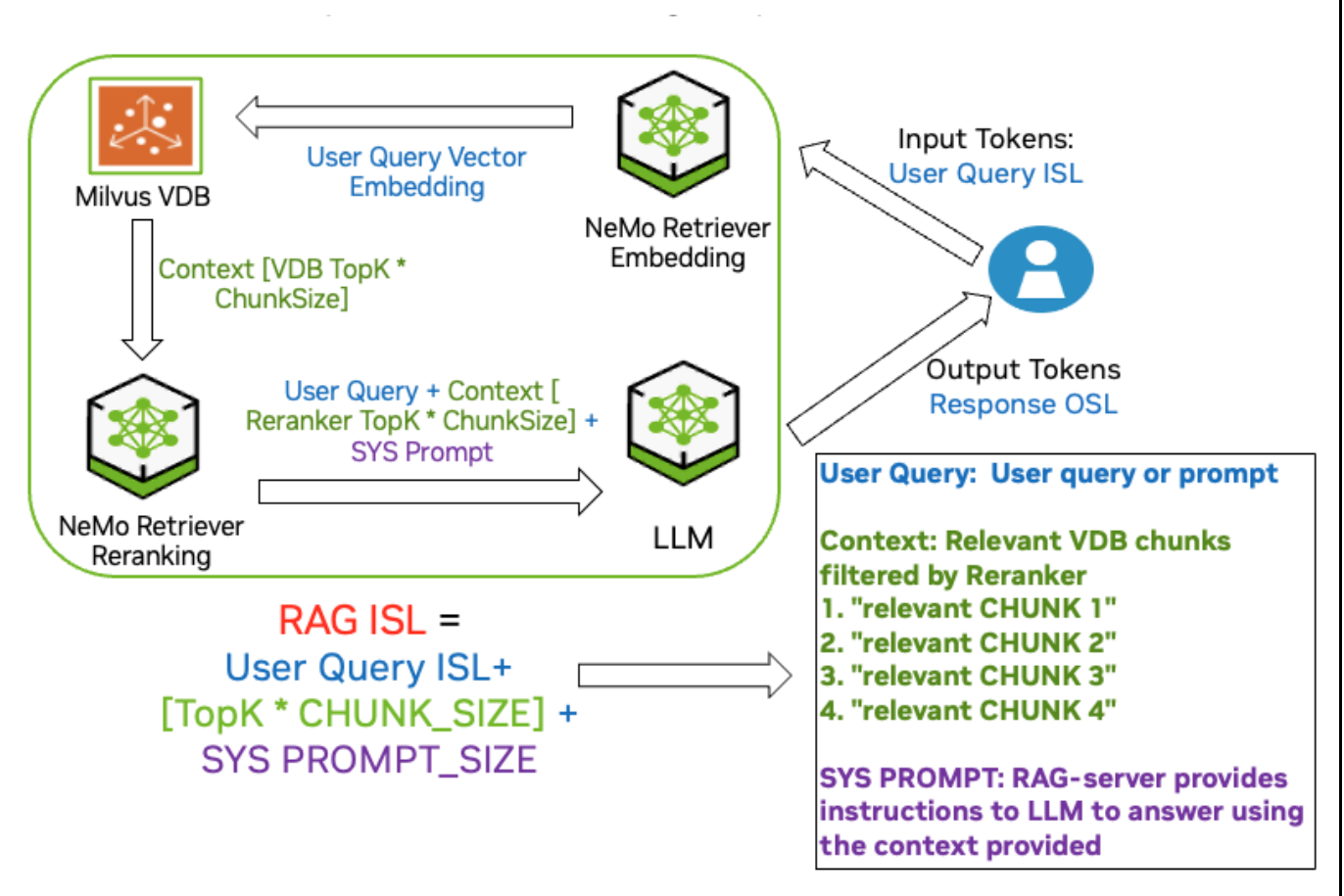
Figure 5 RAG-ON Benchmark

Benchmark	Endpoint	Chat ISL	Description
RAG-OFF	NIM LLM	User Query ISL. For Chat, ISL => 128 tokens	User query (prompt) is sent directly to NIM LLM (skip RAG pipeline completely)

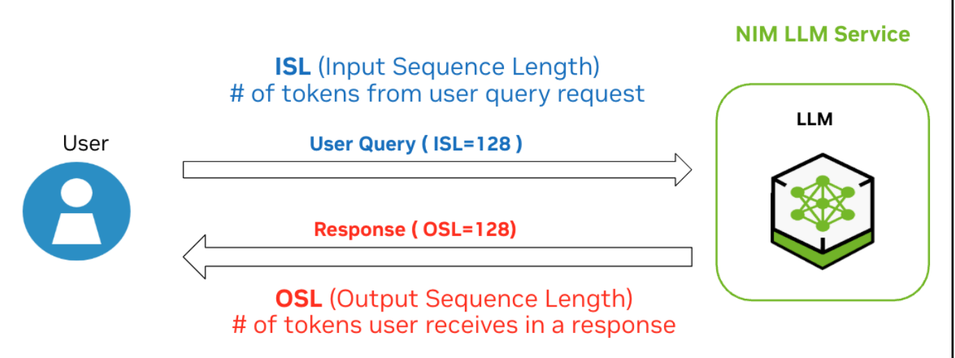
Figure 6 RAG-OFF Benchmark

Benchmark	Endpoint	Chat ISL	Description
RAG-OFF with RAG ISL	NIM LLM	User Query ISL + [TopK * Avg. CHUNK_SIZE] + SYS PROMPT_SIZE. For Chat RAG-ISL = 128 + [4 * 243] + 107 = 1207 tokens	User query (prompt) is sent directly to NIM LLM however the prompt is padded to the ISL that would be received by the LLM if the query were sent to RAG service. This simulates the overhead coming from the longer input sequence length WITHOUT the overhead of the RAG components generating that context. This is the best case or Speed of Light measurement.

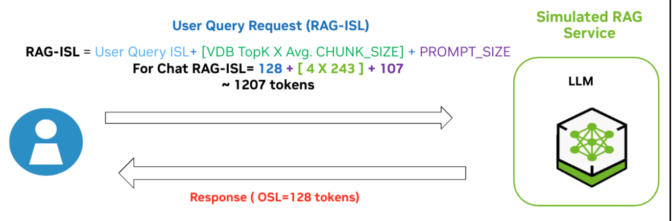
Figure 7 RAG-OFF with RAG-ISL Benchmark

Key Factors affecting Accuracy and Performance

Both Accuracy and Performance are critical for RAG Inference. The primary driver for Enterprise RAG is Accuracy; responses need to be accurate, grounded and relevant to context. There is a constant struggle between Accuracy and Performance, where some metrics that improve accuracy may adversely impact performance. In addition consider the Performance per $ (Cost); this is a measure of cost or revenue generated by the RAG solution. Decisions need to be made on how much accuracy is good enough for each use case in order to not sacrifice performance or increase cost.

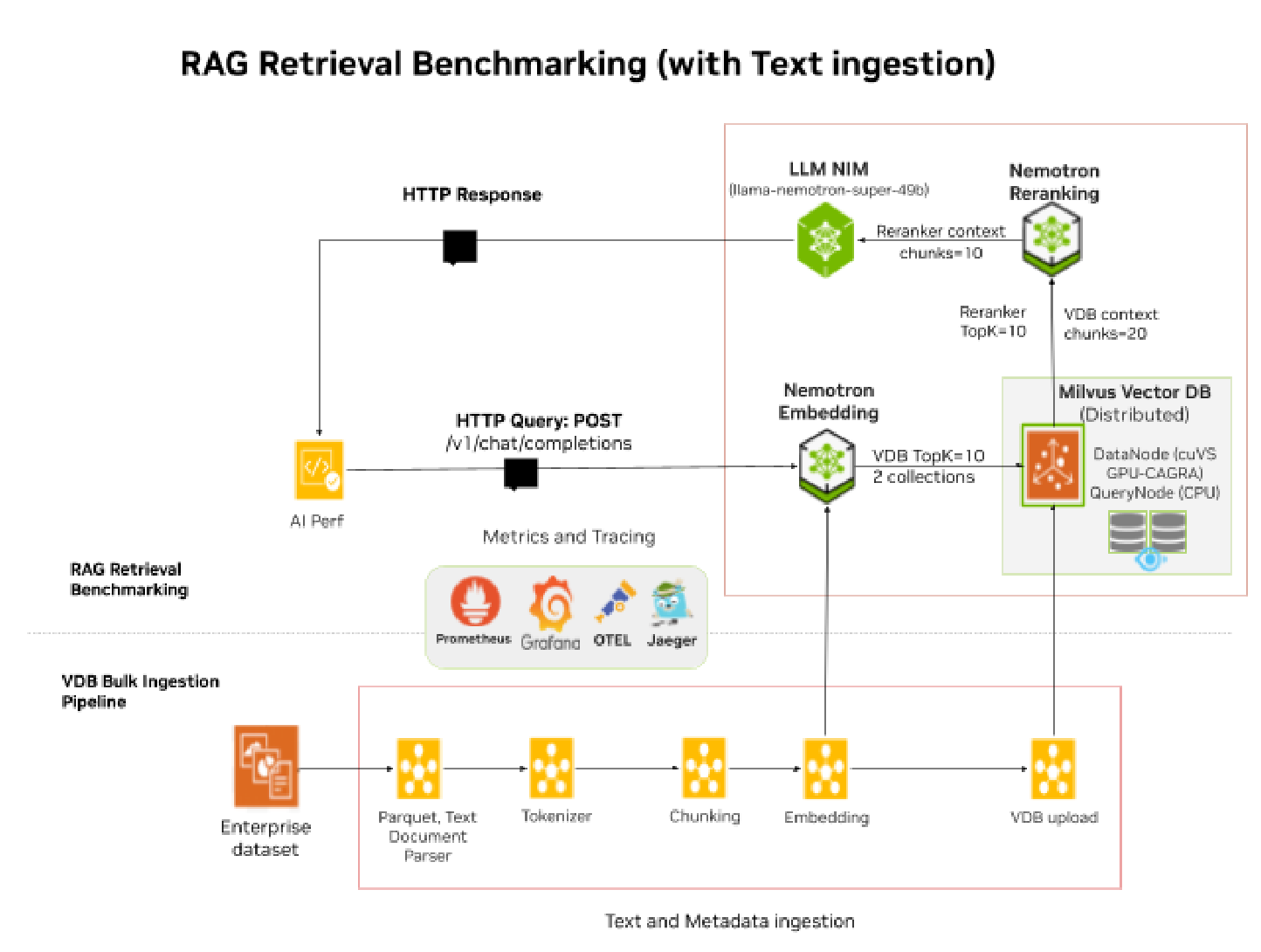
Figure 8 RAG Retrieval Benchmarking Parameters that affect Performance and Accuracy significantly

Performance: LLM Model, GPU, Vector DB scale and GPU acceleration, VDB TopK and Chunk Size, Input Query Length (ISL), Output Response Length (OSL), Reranker TopK.

Accuracy: LLM Model, Chunk Size, Reranker ON/OFF, TopK.

Summary for Key Factors

High level summary of the Enterprise RAG deployment options for Balanced Performance, Accuracy and Performance per GPU ($ Cost).

Parameter	Perf. impact	Accuracy Impact	Cost or Revenue Impact	Enterprise RAG deployment
Hardware GPU	High	NA or Low	High	Enterprise RA 2-8-5 RTX pro 6000, H200 NVL
LLM Model, Engine, Precision, Parallelism	High	High	High	llama-3.3-nemotron-super-49b-v1.5. RTX PRO 6000: vLLM, nvfp4, tp1. H200 NVL: vLLM, fp8, tp1
Vector DB Deployment GPU Mode	High	Low	High	Milvus (Distributed). GPU-CPU Hybrid mode. GPU_CAGRA (cuVS) for Index and CPU for Search
Vector DB Size number of embeddings	Low	NA	Medium	~10M embeddings (2048 dim X FP32) => 80-100 GiB RAM. 2X Data node: 0.5 GPU, 2 X [8 vCPU, 16 GiB RAM]. 2X Query node: 2X [8 vCPU / 40 GiB RAM]
Dataset data type, document size	High (Ingestion)	High	Medium	VDB Bulk ingest => Wikipedia dataset (parquet files) 6M docs. Ingestor-server/NV-Ingest => Shakespeare (44 PDF/text). NV-Ingest Multimodal - digital corpora (bo767 767 pdf)
Reranker ON/OFF	Medium	Medium	High	Ranker ON for benchmarking. Reranker OFF (single collection). Reranker ON for multiple collection search
TopK	High	Medium	High	Chat TopK 10/4 (recommended): Vector DB TopK 10, Reranker TopK 4. Summarization/Generation TopK 20/10 (recommended): Vector DB TopK 20, Reranker TopK 10
Chunk Size (defined at ingest)	High	Low	High	Text Chunk Size: 256/50. Multi-modal Chunk Size: 512/150
Usecase ISL/OSL	High	NA	High	Usecases: Chat: 128/128; Summarization: 2048/512, Analysis: 128/1024

Table 2. Summary RAG Factors affecting Accuracy and Performance

Deep Dive into Key Factors affecting Accuracy, Performance and Cost Efficiency

Let’s dive into these parameters and determine what to use with Enterprise RA RAG solution.

Metric/Parameter	Enterprise RAG Deployment
Cluster Hardware GPU	The choice of GPU has a significant impact on performance and cost. Selecting a Enterprise class GPU: RTX PRO 6000, H200, B200; will provide higher FLOPs, HBM memory, optimized NIM profiles and high performance per $(Cost) => Increased revenue. Enterprise RA 2-8-5 deployed with RTX PRO 6000 and H200 NVL. GPU: H200 NVL 143 GB of HBM3e memory with a 4.8 TB/s. Precision: H200 NVL FP8; RTX PRO 6000 NVFP4. Engine: vLLM. Tensor Parallelism: TP=1 (1 GPU)
LLM Model, Precision	The choice of LLM Model and precision has a significant impact on Accuracy and Performance. The larger models provide better accuracy but reduce performance and increase cost; need more GPUs when using tp2 or higher. Model: llama-3.3-nemotron-super-49b-v1.5 is selected for Enterprise RAG since it supports both bf16 (tp2) and fp8 (tp1) precision and has better overall performance per GPU and accuracy (multi-modal and text benchmarks) than Llama3.1-70b-instruct. nvidia/llama-3.3-nemotron-super-49b-v1.5. Compared with LLMs: Llama3.1-70B-instruct, Llama3.1-8B-instruct. See LLM model accuracy comparison
NIM Cache with Operator	NIM Operator - NIM Cache and NIM Service. NIM Cache provides faster NIM scale out using manual scaling or autoscaling (HPA); ~2-5min (depends on LLM size). Deploy NIM microservices with NIM Operator. coming soon: RAG blueprint support for NIM Operator
Vector DB Deployment GPU mode	Milvus Distributed in GPU-Index and CPU-Search Hybrid mode. Distributed deployment provides independent scaling for Milvus Data and Query nodes in order to support Enterprise level data; ingestion with high document ingest rate >10K documents at a time and support searching multiple collections with high query rate (>50 requests per second). GPU for Index and CPU for Search [Recommended]: GPU CAGRA (cuVS) for Index (Ingest) and then convert to CPU (HNSW) at load time for Search (Retrieval). This hybrid GPU-CPU Milvus provides the benefits of GPU indexing with high performance data ingestion and CPU search that is reasonably efficient at lower query rates (<300 QPS). For baseline enterprise data of <1M vectors, allocate sufficient CPU/Memory for data and query nodes: Data node: 0.25 GPU, 8 vCPU, 8 GiB RAM (Run:ai 25% GPU or MIG RTX PRO 6K mig-1g.24gb). Query node: 8vCPU, 10GiB RAM. Scale out query nodes to support more data, 10GB per 1M tokens. For large enterprise with higher data scale <10M vectors, scale up the data nodes and query nodes and added redundancy: 1-2 X Data node: 1 X 0.25 GPU, 1 X [16 vCPU, 32 GiB RAM]. 2-5 X Query nodes: 2 X [16 vCPU, 40 GiB RAM]
Vector DB Size number of embeddings	Retrieval performance is not significantly affected by using different Vector DB sizes (100K, 500K, 1M, 10M, 20M, 40M embeddings). Large Enterprise Data: 10M-100M vectors (1M-10M documents, 5-50 GB raw text) => vector DB size of 100GB - 1TB. 2-4 Data node: 2 X [0.25 GPU, 16 vCPU, 32 GiB RAM]. 5-10 Query nodes: 5 X [16 vCPU, 40 GiB RAM]. The vectors will be split across multiple collections. All collections don’t have to be loaded in memory simultaneously. You can choose to scale up and scale out the data nodes during ingestion and the query nodes to handle the simultaneous search across multiple collections. There is a 10X penalty Vector DB search latency to load the collection into memory from disk for the first time. Example: 100M Vector DB size (~1 TB, ~10M documents) => 10 collections with 10M vectors or 100 collections with 1M vectors. 100M vector size = 100M X 2048dim X 4B + 20% overhead = ~1 TB
Dataset data type, document size	Data type - PDF Text-only datasets with some tables tend to have better accuracy results than multimodal datasets with images and charts. Document size - large multimodal documents take longer to extract content tables, charts, images. NeMo Retriever Extraction (NV-Ingest) - multimodal documents. For multimodal document ingestion use NeMo Retriever Extraction (NV-Ingest) with Run:ai (time slicing) GPU fractions or Multi Instance GPU (MIG) to extract content tables, charts, images. Use tracing to find the extraction overhead for NV-Ingest NIM microservices and scale up/out the corresponding NIM microservices; typically the Embedding, OCR, page-elements NIM microservices need more resources. Vector DB Bulk Ingest - For text-only parquet documents, e.g. Wikipedia dataset parquet files. Use multi-threaded python script to parse, tokenize, chunk, embed and then bulk ingest data directly into Milvus. Enterprise datasets: Basic validation - Ingestor server for PDF text-only: Shakespeare dataset => 44 documents, 9K embeddings. Wiki Text-only Vector DB bulk ingest for parquet text-only: Wikipedia dataset (parquet files) => 5.9 M documents, 38M vector embeddings (chunk size 256/50, 2048dim X FP32). NeMo Retriever Extraction for Multimodal PDF dataset: with text, table, charts, images e.g. digital corpora (bo767) => 767 PDFs; 77K embeddings (pages: 54730, tables: 23323, total_charts: 7835, elements: 85,888). See also: digital_corpora_download.ipynb
Reranker ON/OFF	Reranker adds ~10% overhead to First Token Latency. Reranker is effective to filter data from multiple collections. Reranker improves Accuracy by 3%-10% for multi-modal datasets. Reranker adds to the overall cost of the RAG solution, and increases the cost in terms of performance per GPU since it needs to be scaled with the LLM using scale ratio 1:2 or 1:4 depending on use case. For Summarization (1024/512) use cases with large Input Query length (ISL=1024) and large context from Vector DB TopK>10, the Reranking NIM load increases by 2-4X and needs at 1:2 scale ratio with respect to LLM. See reranker accuracy comparison
VDB / Reranker TopK	VDB TopK and Reranker TopK define the number of vector chunk data sent to the LLM as Context. Increasing the TopK from 4 => 10, increases the Context overhead by 2.5 times, and increases First Token Latency by 2X or higher, and increases the Accuracy by 3%-9% for multi-modal datasets. For Enterprise RAG with Reranker ON: Chat (128/128): VDB TopK/ Reranker TopK 10/4. Summarization (1024/512): VDB TopK/ Reranker TopK 20/10. See TopK accuracy comparison
Chunk Size (defined at ingest)	Chunk Size and overlap are selected at ingestion, when ingesting data into the Vector DB and cannot be changed after that. The document to be ingested is split into smaller chunks based on Chunk Size (tokens) and Overlap(tokens) before it is vectorized into embeddings and stored in the vector DB. Overlap is the amount of overlapping tokens from the previous chunk that is included in the current Chunk to maintain context. Overlap is usually 10%-20% of the Chunk Size. Has a significant impact on performance and using larger chunks can increase accuracy up to a certain point especially for multi-modal data. For Chat use cases with text-only data, varying Chunk Size has little or no effect (<1%). Increase Chunk size from 512/150 to 1024/150 tokens results in: Accuracy => Low Impact, Performance => High Impact. Accuracy increases by 2%-5% for some multi-modal datasets when increasing ChunkSize from 256 to 512. For Chat (128/128) use case; increasing ChunkSize from 256 to 512 tokens: increases RAG-ISL by ~2X, ~1000 tokens, Throughput (TPS) decreases by 1/4 X - 1/3 X (25% - 33%), Latency (TTFT) increases 1.5x - 2x (50%-100%). Chunk Size selection depends on the use case; for research assistant or root cause analysis use cases it may make sense to use larger chunk size. To reduce the performance impact of Chunk Size select smaller chunk sizes but increase TopK and send chunks to Reranker to filter some out before sending to the LLM. For Enterprise RA, selected Chunk Size of 256, since the focus was Retrieval Performance with text-only data. Chunk Size: 256/50 => 256 tokens + 50 tokens overlap; Average chunk size: 243 tokens (From tracing data for Shakespeare dataset); Used for calculating the RAG-ISL for simulated RAG validation. Recommendation: Chunk size 256/50 for text-only data for best performance and accuracy combined. See chunk size accuracy comparison
Usecase ISL/OSL	RAG Retrieval Performance use cases require standardization for ISL and OSL and use synthetic dynamic data in order to create multiple requests for different concurrent users and calculate the First Token Latency percentile over 100s of requests. Chat: 128/128; Summarization: 1024/512, Generation: 128/2048. Accuracy benchmarking relies on Evaluation datasets where the queries and responses are fixed; typically short ISL and OSL but the length of response can vary. There is an effort underway to use the same evaluation datasets for both Accuracy and Performance benchmarking. The ISL and OSL will vary and need to determine an average ISL and OSL for each dataset. In addition the number of queries available in the evaluation dataset is fixed and not very large. When running performance benchmarking with a large number of concurrent users, there could be query repetition and KV-Cache hits that would show much lower than expected latency. Cannot validate Summarization and Analysis use cases with longer ISL/OSL, since evaluation data sets have shorter ISL/OSL, short query with short response.

Table 1. Details RAG Factors affecting Accuracy and Performance

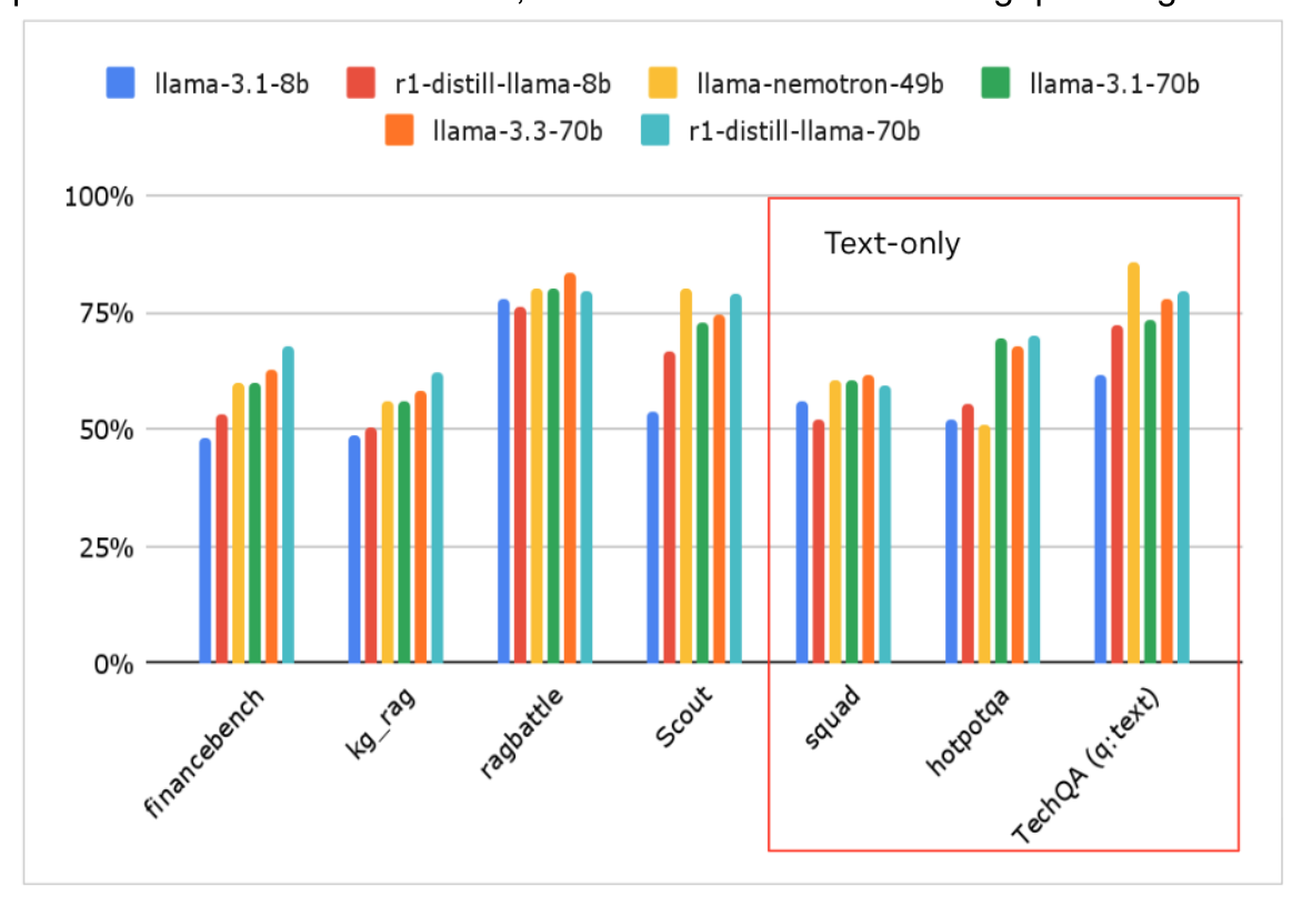
Figure 9 LLM Model Accuracy Comparison Across Benchmarks

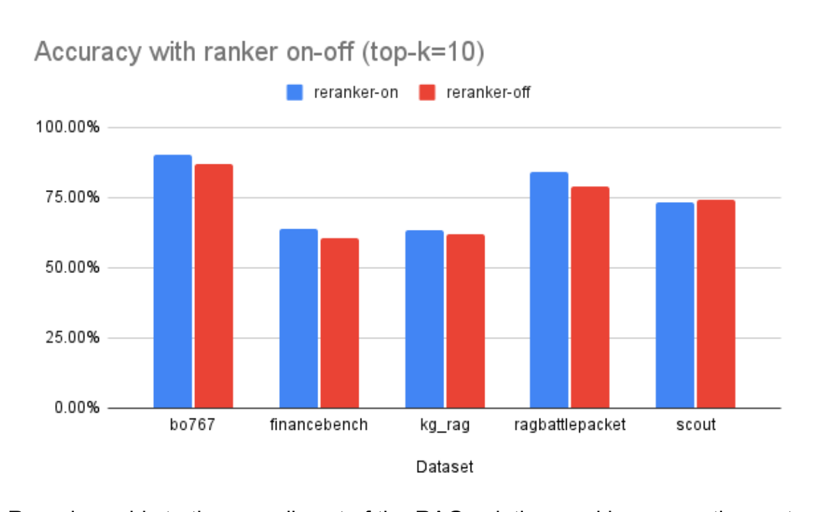
Figure 10 Accuracy with Reranker ON vs OFF (top-k=10)

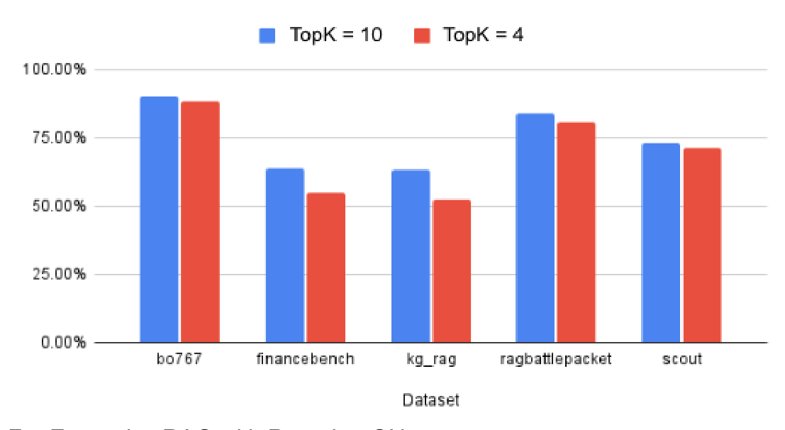
Figure 11 Accuracy Impact of TopK: TopK=10 vs TopK=4

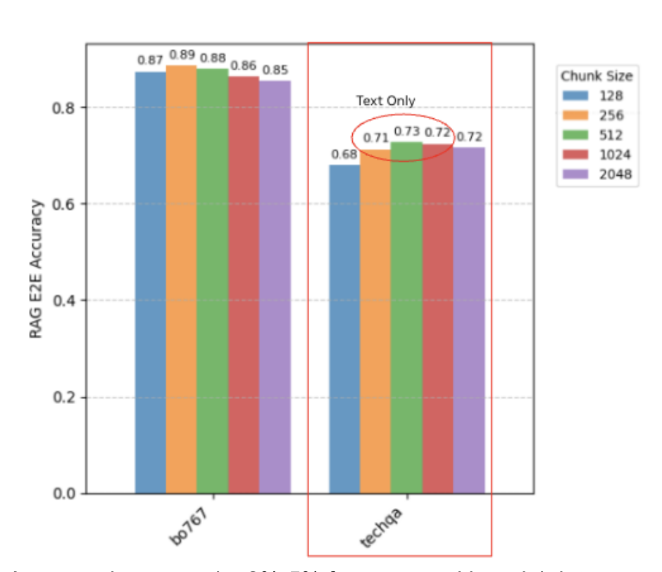
Figure 12 Chunk Size Impact on RAG E2E Accuracy

Chunk Size Impact on Latency

Chunk Size can have a significant impact on performance; for the chart below Chunk Size is varied: 256 tokens vs 512 tokens vs 1024 tokens.

For Concurrent Requests (users) CR=30, the First Token Latency increase by ~2X as the Chunk Size increases by 2X (256 to 512 and 512 to 1024):

• Chunk Size 256, TTFT=~2s

• Chunk Size 512, TTFT=~3.8s

• Chunk Size 1024, TTFT=~7.1s

And for TTFT=2s, the Concurrent Requests decrease by ~50%:

• Chunk Size 256, CR=~30

• Chunk Size 512, CR=~15

• Chunk Size 1024, CR=~8

Model and Chunk Size Impact on Throughput (RPS)

Here the Output Throughput performance is being compared for different models (Llama-3.1-8b, Llama3.1-70b and Llama-Nemotron-49b) along with different chunk sizes.

For Chat use case LLM Scale 1X, the smallest model Llama-3.1-8b (precision FP8 TP1 with 1 GPU) and smallest chunk size=128 tokens shows maximum throughput = ~15 RPS (Requests per second). Even with LLM Scale 50X the best case maximum throughput for RAG Retrieval will not exceed 50 X 15 = 750 RPS.

Llama-Nemotron-70b with ChunkSize=256, has a maximum throughput=~5 RPS, at LLM Scale 50X the best case maximum throughput for RAG Retrieval will not exceed 50 X 5 = 250 RPS.

The output throughout (RPS) drops significantly from 15 RPS to 5 RPS (by 1/3) when using larger models Llama-3.1-70b and Llama-Nemotron-70b.

Llama-3.1-70b with Chunk Size=128 (Blue line) has throughput ~6 RPS which is 2 times higher throughput than Llama-3.1-70b with Chunk Size=512 (Red line) ~3 RPS.

Increasing the Chunk Size from 128 tokens to 512 tokens with TopK=4 causes the ISL to increase by ~1500 tokens which will result in substantial (>50%) drop in output throughput at the Maximum Throughput region on the graph.

TopK and Reranker ON/OFF Impact

Reranker Impact on Throughput

From the chart below, enabling the reranker impacts both the raw Output throughput (Tokens per second) as well as the Per User Throughput (TPS) especially at the lower concurrencies Concurrency CR<30. At higher concurrencies the throughput impact is not as prominent (red and blue lines merge).

Latency sensitivity Chat applications requiring TTFT <3s run at lower concurrencies CR <=20 and are more likely to have performance impacted by the addition of the Reranker.

Reranker Impact on Latency

For Latency sensitive use cases, Low Latency TTFT <3s or Very Low Latency TTFT<1s constraints, the Latency impact from the Reranker may be more prominent.

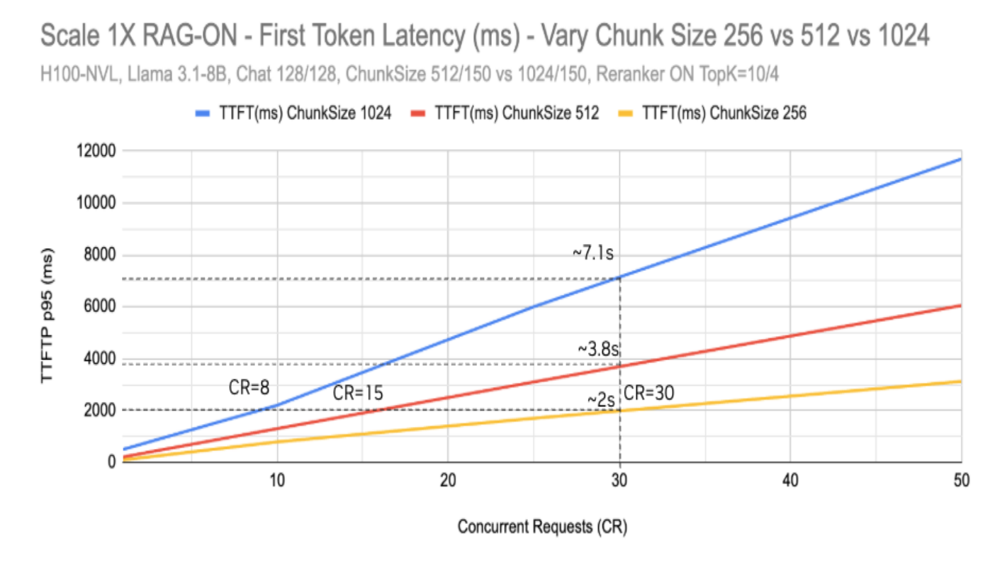
Figure 13 Reranker Impact on First Token Latency (TTFT)

VDB TopK Impact on Latency

Usecase - RAG Scale 1X, Chat 128/128, Reranker OFF:

• VDB TopK = 4

• VDB TopK = 10

This use case depicts the impact of Vector DB TopK selection on Latency; VDB TopK can improve Accuracy but also has a significant impact on First Token Latency (TTFT). Increasing the VDB TopK from 4 to 10 increases the context (data chunks) that is sent to LLM (RAG ISL) by 2.5 times. The ISL increases by ~1450 tokens for Chunk Size 256.

Let’s look at some data points on the Latency chart below comparing different VDB TopK.

At Concurrent Requests CR=40, the First Token Latency is more than 2 times for VDB TopK=10 vs VDB TopK=4:

• RAG-ON Reranker OFF, VDB TopK=4, TTFT = ~3.6s

• RAG-ON Reranker OFF, VDB TopK=10, TTFT = ~7.9s

At Time to First Token TTFT =5s, the Concurrent Requests is more than double times for VDB TopK=4 vs VDB TopK=10:

• RAG-ON Reranker OFF, VDB TopK=10, CR = 25

• RAG-ON Reranker OFF, VDB TopK=4, CR = 56

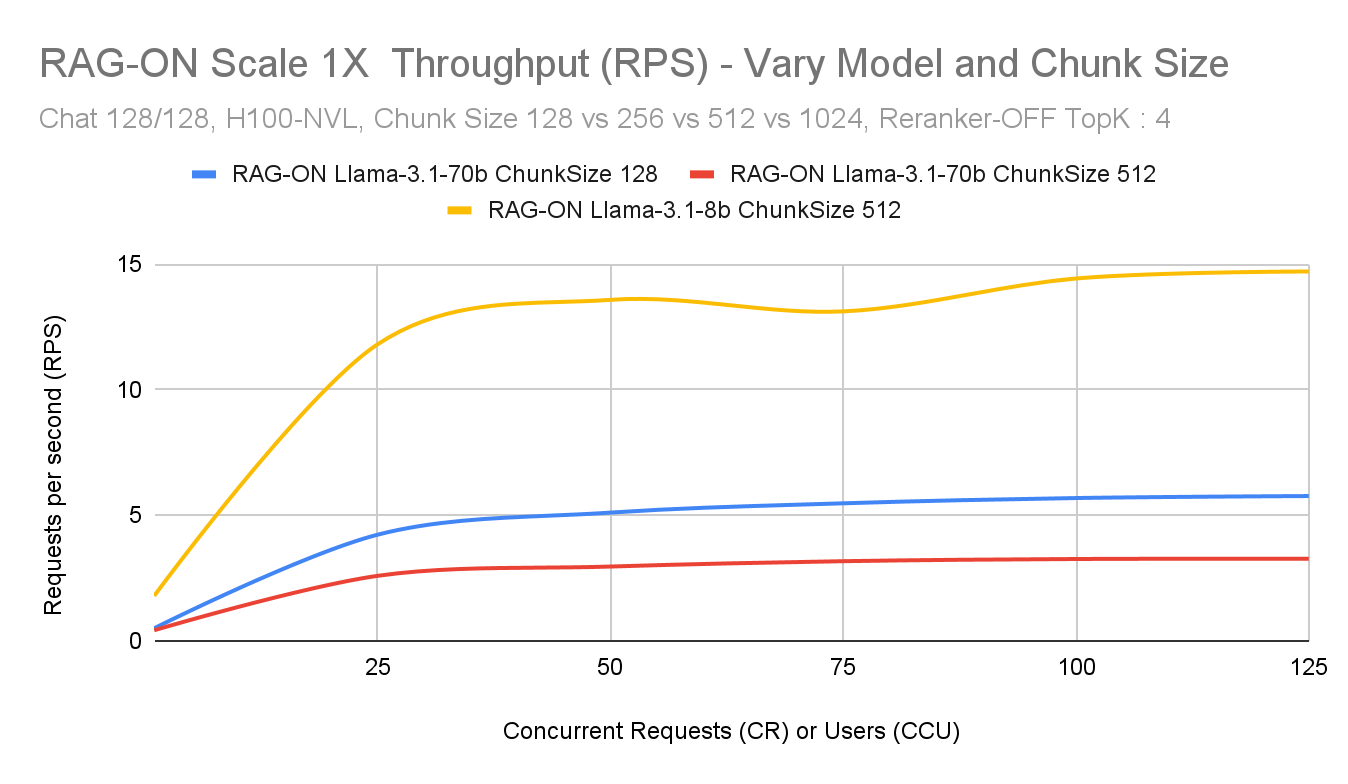
Figure 14 VDB TopK Impact on First Token Latency (TTFT)

VDB TopK Impact on Output Throughput

Usecase - RAG Scale 1X, Chat 128/128, Reranker OFF.

For the Output Throughput chart below comparing different TopK with Reranker ON and OFF:

At Concurrent Requests CR=20, the Output Throughput for VDB TopK=10 vs VDB TopK=4 drops by more than 1/3:

• RAG-ON, Reranker OFF, VDB TopK=4, Output Throughput = 379 TPS

• RAG-ON, Reranker OFF, VDB TopK=10, Output Throughput = 241 TPS (36.33% decrease)

At Concurrent Requests CR=50, the Output Throughput for VDB TopK=10 vs VDB TopK=4 drops by more than 45%:

• RAG-ON Reranker OFF, VDB TopK=4, Output Throughput = 533 TPS

• RAG-ON Reranker OFF, VDB TopK=10, Output Throughput = 285 TPS (46.61% decrease)

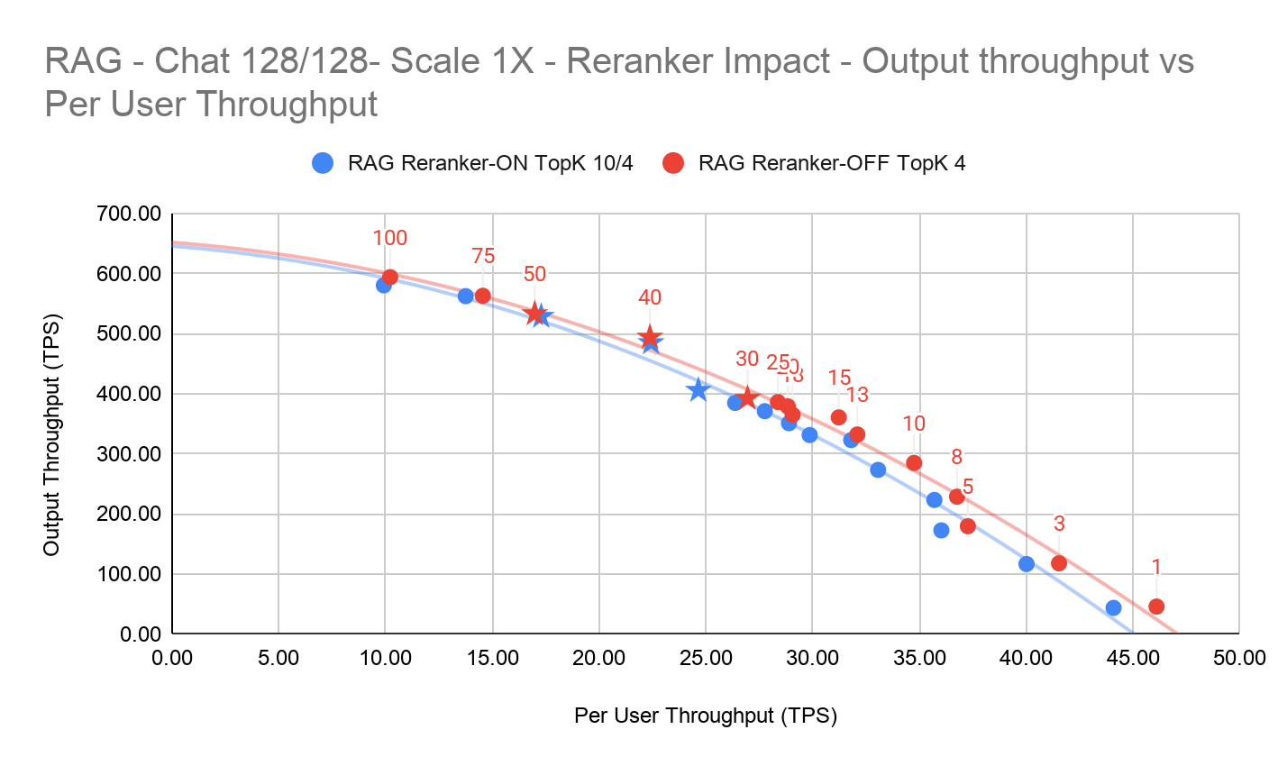
Figure 15 VDB TopK Impact on Output Throughput (TPS)

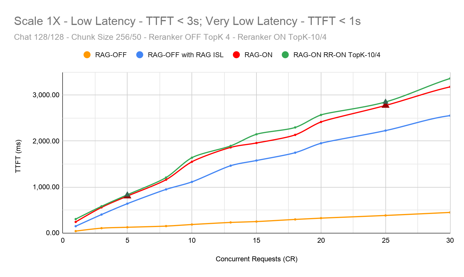
Figure 16 VDB TopK Impact on Output Throughput - Detailed Comparison

Latency Benchmark - Usecase Chat 128/128, Reranker ON, Vary TopK

• RAG ON, Reranker ON, VDB TopK = 10, Reranker TopK=4

• RAG ON, Reranker ON, VDB TopK = 20, Reranker TopK=4

This use case depicts the impact of enabling the Reranker on Latency. The Reranker can improve Accuracy especially when querying multiple collections with multi-modal data to filter out less relevant context. But it has an impact on performance per $ (cost); scale the Reranker along with the LLM.

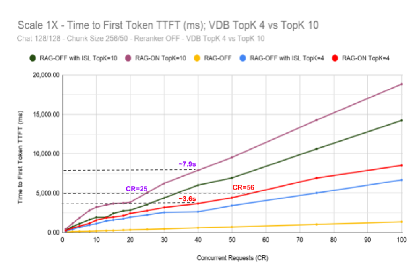
Figure 17 Latency Benchmark - RAG Chat 128/128, Reranker ON, Varying TopK

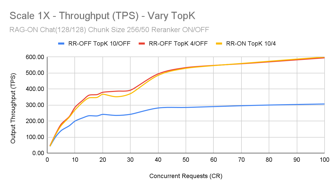
Figure 18 TTFT Impact from Reranker and VDB TopK Variation

Adding the Reranking NIM adds a small <10% latency overhead to Time to First Token (TTFT). However the Reranker needs to be scaled in sync with the LLM (1:8 ratio for Chat) in order to maintain <10% overhead on TTFT, this decreases the performance per $ (TCO cost).

Increasing the VDB TopK from 10 to 20 adds a very small overhead (<1% of TTFT) to Retriever Milvus VDB.

In summary:

Reranker should only be enabled when context from multiple collections need to be filtered to reduce overhead on the LLM.

Increasing ISL by ~1400 tokens results in the RAG Throughput drops by 36%-46%.

In Summary for every 1000 tokens additional overhead to ISL, the RAG Output Throughput drops by:

• up to 25% for Low Latency range TTFT <3s

• up to 33% for Balanced Performance range; 3s < TTFT <5s

• close to 50% for Max. Throughput range TTFT >5s

Additional ISL overhead can come from increasing ChunkSize from 256 to 512 or from increasing TopK from 4 to 10.

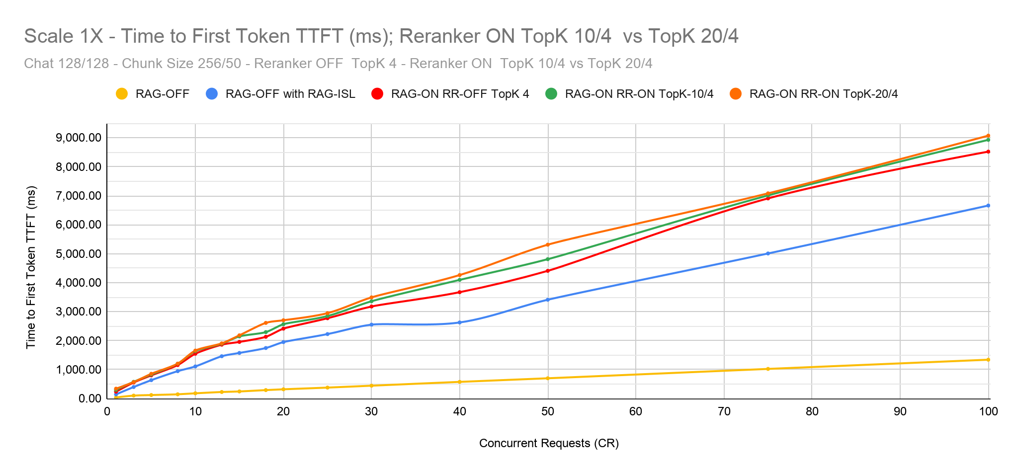
Figure 19 Summary: ISL Increase Impact on RAG Output Throughput across Latency Ranges