2. Interactive Workload Examples#

In this section, we give instructions for running several Workloads on your DGX Cloud Create cluster. The examples are not exhaustive, but can be adapted for your own workloads.

2.1. Interactive NeMo Workload Job#

In this example, we step through the process of creating an interactive workload using the NeMo container from NGC. Interactive workloads in NVIDIA Run:ai are called Workspaces. In this particular example, we will run a Jupyter notebook to fine-tune an LLM (Llama3-8B Instruct) using LoRA against the PubMedQA dataset.

2.1.1. Prerequisites and Requirements#

The following are required before running the interactive NeMo job:

You must have accepted an invitation to your NGC org and added your NGC credentials to the NVIDIA Run:ai. See details here.
You must have the user role L1 researcher, ML Engineer, or Application Administrator to run through all sections of this tutorial.
Your user must be able to access a project and department.
You must have access to a compute resource with at least one GPU with 80 GB of memory created in your scope that you can use.
You must create a Hugging Face account and agree to the Meta Llama 3 Community License Agreement while signed in to your Hugging Face account. You must then generate a Hugging Face read access token in your account settings. This token is required to access the Llama3 model in the Jupyter Notebook.

2.1.2. Creating the Data Source#

To make it easier to reuse code and checkpoints in future jobs, a persistent volume claim (PVC) is created as a data source. The PVC can be mounted in jobs and will persist after the job completes, allowing any generated data to be reused.

To create a new PVC, go to the Data Sources page. Click New Data Source and then PVC to open the PVC creation form.
On the new form, set the desired scope.

Important

PVC Data Sources created at the cluster or department level do not replicate data across projects or namespaces. Each project or namespace will be provisioned as a separate PVC replica with different underlying PVs; therefore, the data in each PVC is not replicated.
Give the PVC a memorable name like nemo-lora-checkpoints and add a description if desired.
For the data options, select a new PVC storage class that suits your needs according to the PVC recommendations here. In this example, dgxc-enterprise-file is sufficient. To allow all nodes to read and write from/to the PVC, select Read-write by many nodes for the access mode. Enter 10 TB for the size to ensure we have plenty of capacity for future jobs. Select Filesystem as the volume mode. Lastly, set the Container path to /checkpoints, where the PVC will be mounted inside containers. This completed section should look as shown below.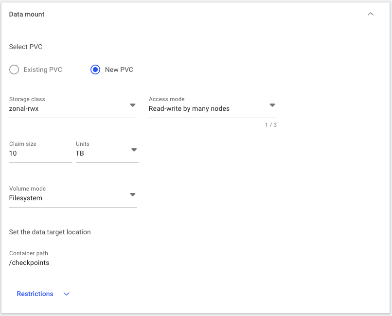
Once the form is complete, create the data source using the button at the bottom of the page.

Note

The first time a job is launched using a new PVC, it will take longer to start as the storage gets provisioned only once the first claim to the PVC is made.

2.1.3. Creating the Workspace#

With the PVC created, we can configure the workspace to tell NVIDIA Run:ai how the job should be launched. To do so, go to the Workloads overview page and click the + New Workload button in the top left. A drop-down menu will appear. From the drop-down menu, select Workspace. You will be taken to the New workspace creation page.
Select the desired project to run your job in.
Leave the Template pane of the form set to Start from scratch.
Enter a descriptive name for your Workspace, such as nemo-pubmedqa-lora. Click Continue. After a few seconds the Environment pane of the creation process will appear.
The environment is a template with common settings that can be reused for similar jobs. For example, an environment might be based on a PyTorch container and have Jupyter exposed as a tool enabling anyone who needs to run interactive PyTorch jobs inside a Jupyter notebook to use the same template instead of launching unique jobs and re-configuring the settings each time they want to experiment. In this example, a new environment will be created based on the NeMo container and expose Jupyter as a tool to make it easier to reuse the template in the future.
To create a new environment for the NeMo job, click the + New Environment button in the top right of the Environment pane. The Environment creation form will open.
In the Environment creation form, enter a name for the environment, such as “nemo-jupyter” and optionally add a description.
Under Image URL, put nvcr.io/nvidia/nemo:25.02. This pulls the NeMo container from NGC. If desired, the image pull policy can be changed. The default value of “if not already present” is recommended for most cases, but if you are pushing new containers to the NGC org with the same tag, “always pull the image from the registry” should be used to check if there are updates to the image.
Under the Workload architecture & type pane, select Standard and Workspace if they are not selected already. These options are likely already selected and grayed out.
Click the Tools pane to open the tools menu, and click +Tool. This list allows you to add additional tools to the workspace to make it easier to connect to their resources, such as Jupyter for connecting to external Jupyter lab sessions, VS Code for connecting to VS Code servers inside the job, and more.
Since we want to run an interactive Jupyter notebook, select Jupyter in the Select tool list. The Connection type drop-down should show External URL, Auto generate and Container port “8888”.
Click the Runtime settings pane, then click to expand the commands and arguments pane. This section allows us to override the default container run settings as needed. Since we want to launch a Jupyter lab session, enter jupyter-lab as the command, and --NotebookApp.base_url=/${RUNAI_PROJECT}/${RUNAI_JOB_NAME} --NotebookApp.token='' --ServerApp.allow_remote_access=true --allow-root --port=8888 --no-browser for the arguments. This tells NVIDIA Run:ai how to connect to the Jupyter lab session in the UI.
For the directory, specify /opt/NeMo as the directory to launch the job in. This will launch the Jupyter lab session inside the /opt/NeMo directory inside the container.
Click Create Environment in the bottom right of the page. You should see a pop-up saying that your environment has been created. The page will refresh, and you will be taken back to the top of the Environment pane of the New workspace creation page. The environment you just created should now be selected.
Go to the Compute resource pane and select a single-GPU compute resource for your environment. While it is possible to use more GPUs for LoRA, most tasks can be completed with just a single Ampere or newer GPU with 80GBs of memory in a relatively short period.
In the Data Sources section, select your nemo-lora-checkpoints PVC.
Go to the bottom of the page and click Create Workspace. This will add your job to the queue and it will automatically get scheduled once cluster resources are available.
After creating the workspace, you will be taken to the workload overview page, where you can view the status of your workload. Your interactive workload is ready once the status reads “Running”. This may take a while if the container you chose has not previously been pulled to the cluster and the PVC needs to be provisioned for the first time.
Once the status is “Running”, you can launch the Jupyter lab session by selecting the checkbox next to your workload and clicking CONNECT → Jupyter on the top menu bar. Jupyter lab will open in a new window.

2.1.4. Running the Notebook#

Once connected to the Jupyter lab session, navigate to the example notebook by opening to the tutorials/llm/llama/biomedical-qa directory inside the /opt/NeMo folder the container automatically opens to. Inside this directory are a couple of notebooks, including llama3-lora-nemofw.ipynb, which is the one we will be following. Double-click that file to open the notebook on the main screen.

The notebook walks through what each step does, but at a high level, it does the following:

Downloads the Llama3-8B Instruct model from Hugging Face
Converts the model to the .nemo format to be easily ingested by the NeMo toolkit
Downloads and preprocesses the PubMedQA dataset
Fine-tunes the Llama3-8B Instruct model using the LoRA PEFT technique against the PubMedQA dataset
Deploys the model for local inference
Evaluates the model against the test dataset to determine the overall accuracy of the fine-tuned model

The notebook can be stepped through cell-by-cell or run all at once, and the results viewed later. The only important note is that cell 2 requires you to add your Hugging Face access token, as listed in the requirements section in the cell text, in order to authenticate with Hugging Face to download the model.

As the notebook runs, you can navigate back to the NVIDIA Run:ai workloads page, where your job now shows metrics based on your resource usage. The metrics tab shows the GPU and CPU compute and memory usage during the job. This is a great resource for determining how your job is performing.

2.1.5. Persisting the Model to Storage#

As the PVC was added to the workspace and is mounted at /checkpoints inside the container, any files or directories that are saved to /checkpoints inside the container will be saved in the PVC and available in future jobs.

To save the generated model to the PVC, open a terminal tab inside the Jupyter lab session and navigate to the notebook directory with:
```
cd /opt/NeMo/tutorials/llm/llama-3
```

The model is saved at results/Meta-Llama-3-8B-Instruct/checkpoints/megatron_gpt_peft_lora_tuning.nemo. It can be verified with:

$ du -sh results/Meta-Llama-3-8B-Instruct/checkpoints/megatron_gpt_peft_lora_tuning.nemo

21M     results/Meta-Llama-3-8B-Instruct/checkpoints/megatron_gpt_peft_lora_tuning.nemo

To copy the file to the PVC, run:

cp results/Meta-Llama-3-8B-Instruct/checkpoints/megatron_gpt_peft_lora_tuning.nemo /checkpoints

Once the checkpoint is copied, it will be available in all future workloads that use that same PVC unless the file is intentionally removed.

2.1.6. Cleaning up the Environment#

After the job finishes, it can be deleted to free up resources for other jobs. Note that certain jobs do not self-terminate and should be monitored to ensure resources are not idle for completed jobs.

2.2. RAPIDS and Polars Workspace#

In this example, we step through the process of creating another Workspace, which uses the RAPIDS container from NGC. We will launch a Jupyter environment to experiment with the new integration between RAPIDS and Polars.

2.2.1. Prerequisites and Requirements#

The following are required before running the RAPIDS workspace:

You must have the user role L1 researcher, ML Engineer, or Application Administrator to run through all sections of this tutorial.
Your user must be able to access a project and department.
At least one idle GPU within your DGX Cloud Create cluster.
You must have access to a compute resource with at least one GPU created in your scope that you can use.

2.2.2. Creating the Workspace#

Go to the Workloads overview page and click the + New Workload button in the top left. A drop-down menu will appear. From the drop-down menu, select Workspace. You will be taken to the New workspace creation page.
Select the desired project to run your job in.
Leave the Template pane of the form set to Start from scratch.
Enter a descriptive name for your Workspace, such as rapids-polars. Click Continue. After a few seconds the Environment pane of the creation process will appear.
To create a new environment for the RAPIDS workspace, click the + New Environment button in the top right of the Environment pane. The Environment creation form will open.
In the Environment creation form, enter a name for the environment, such as “rapids-jupyter” and optionally add a description.
Under Image URL, put nvcr.io/nvidia/rapidsai/notebooks:24.08-cuda11.8-py3.9. If desired, the image pull policy can be changed. The default value of “if not already present” is recommended for most cases but if you are pushing new containers to the NGC org with the same tag “always pull the image from the registry” should be used to check if there are updates to the image.
Under the Workload architecture & type pane, select Standard and Workspace if they are not selected already. These options are likely already selected and grayed out.
Click the Tools pane to open the tools menu, and click +Tool. This list allows you to add additional tools to the workspace to make it easier to connect to their resources, such as Jupyter for connecting to external Jupyter lab sessions, VS Code for connecting to VS Code servers inside the workspace, and more.
Since we want to run a Jupyter notebook, select Jupyter in the Select tool list. The Connection type drop-down should show External URL, Auto generate and Container port “8888”.
Click the Runtime settings pane, then click to expand the commands and arguments pane. This section allows us to override the default container run settings as needed. Since we want to launch a Jupyter lab session, enter jupyter-lab as the command, and --NotebookApp.base_url=/${RUNAI_PROJECT}/${RUNAI_JOB_NAME} --NotebookApp.token='' --ServerApp.allow_remote_access=true --allow-root --port=8888 --no-browser for the arguments. This tells NVIDIA Run:ai how to connect to the Jupyter lab session in the UI.
Do not modify any other settings.
Click Create Environment in the bottom right of the page. You should see a pop-up saying that your environment has been created. The page will refresh, and you will be taken back to the top of the Environment pane of the New workspace creation page. The environment you just created should now be selected.
Go to the Compute resource pane and select a single GPU compute resource for your environment.
Go to the bottom of the page and click Create Workspace. This will add your job to the queue and it will automatically get scheduled once cluster resources are available.
After creating the workspace, you will be taken to the workload overview page, where you can view the status of your workload. Your workspace is ready once the status reads “Running”. This may take a while if the container you chose has not previously been pulled to the cluster.
Once the status is “Running”, you can launch the Jupyter lab session by selecting the checkbox next to your workload, and clicking CONNECT → Jupyter on the top menu bar. Jupyter lab will open in a new window.

2.2.3. Downloading the Polars Notebook#

Once connected to the Jupyter lab session, you can navigate to the integrated RAPIDS notebook samples within the notebooks directory and experiment within your workspace.

To get started downloading the GPU-accelerated Polars example notebook, open a terminal interface by clicking the Terminal box.

In the resulting terminal, run the following command to download the new notebook.

wget https://raw.githubusercontent.com/rapidsai-community/showcase/refs/heads/main/accelerated_data_processing_examples/polars_gpu_engine_demo.ipynb

2.2.4. Running the Polars Notebook#

The notebook provides an introduction to what Polars is and where it is best used, along with code to:

Install Polars with GPU Engine, along with other notebook dependencies
Download a sample Kaggle dataset
Initialize Polars to use the GPU in DGX Cloud Create
Run various sample analyses to provide performance comparisons between Polars with CPU only and Polars with GPU

To open the notebook, double-click on the file named polars_gpu_engine_demo.ipynb when it becomes visible in the Jupyter file navigation pane.

The notebook can be stepped through cell-by-cell or run all at once, and the results can be viewed later.

As the notebook is running, you can navigate back to the NVIDIA Run:ai workloads page, where your job now shows metrics based on your resource usage. The metrics tab shows the GPU and CPU compute and memory usage during the job. This is a great resource for determining how your job is performing. Within the Jupyter notebook page you are using, you can also use an integrated GPU performance visualization plugin from the RAPIDS NGC container (it is the tab on the left side of the page with a GPU icon on it).

2.2.5. Cleaning up the Environment#

After you are finished with the workload, it can be stopped or deleted to free up resources for other workloads. Note that certain workloads do not self-terminate and workloads should be monitored to ensure resources are not sitting idle for completed workloads.

2.3. Running Visual Studio Code Server#

In this example, we step through the process of creating a Workspace via the NVIDIA Run:ai Command-Line Interface (CLI) that runs a VS Code instance, and exposing the necessary port to our local workstation in order to access the VS Code web interface.

2.3.1. Prerequisites and Requirements#

The following are required before running the VS Code workspace:

You must have the user role L1 researcher, ML Engineer, or Application Administrator to run through all sections of this tutorial.
Your user must be able to access a project and department.
You must have installed the NVIDIA Run:ai CLI tool, as detailed in the Advanced documentation.

2.3.2. Creating the Workspace via CLI on a local workstation#

Open a terminal on your workstation (or other system that has the NVIDIA Run:ai CLI installed and configured on it).

Note

If the system you have installed the NVIDIA Run:ai CLI on is a remote system, you can SSH to that system and create a local port forward, connecting the port NVIDIA Run:ai will use with the same port on your local workstation. For example, ssh -L 8080:localhost:8080 the-ip-or-hostname-of-your-remote-system.
Make note of your target project.

Enter the following command and arguments into your terminal (inserting your target project as the argument to the --project flag) and hit enter.

runai submit vscode --project your-project-name-here --image linuxserver/code-server:4.92.2 --environment PUID=0 --environment PGID=0 --interactive

(Optional) Validate that the workload is running with the following command.
```
runai describe job vscode --project your-project-name-here
```
Forward a port to your local workstation through the NVIDIA Run:ai CLI with the following command. The first port in the argument to port is arbitrary - it can be changed to any unused port on your system, instead of 8080.
```
runai port-forward vscode --project your-project-name-here --port 8080:8443
```
To access the VS Code web interface, navigate to http://localhost:8080.

2.3.3. Cleaning up the Environment#

After you are finished with the workload, it can be stopped or deleted to free up resources for other workloads. To delete the workload from the CLI, use the following command.

runai delete --project demo-project job vscode

2.4. Building and Running an Interactive PyTorch Job with Visual Studio Code#

In this example, we will create a container with an SSH server running within it, and launch that container as an interactive Workload which we will then connect to using Visual Studio Code. We will then run a sample python script within Visual Studio to train a ResNet-50 model.

2.4.1. Prerequisites and Requirements#

You must have accepted an invitation to your NGC org and added your NGC credentials to NVIDIA Run:ai. See details here.
You must have the user role L1 researcher, ML Engineer, or Application Administrator to run through all sections of this tutorial.
Your user must be able to access a project and department.
At least one idle GPU within your DGX Cloud Create cluster.
You must have access to a compute resource with at least one GPU created in your scope that you can use.
You must have the NVIDIA Run:ai CLI set up and logged in. See details here.

2.4.2. Creating and Using a Custom Docker Container#

In order for this example to function, we require a container image with an SSH server installed.

To create a container, you’ll need to run the following commands on an x64_64-based Linux system or workstation with the Docker container engine installed and authenticated with your NGC account using your API key. For more instructions on how to set this up, see the NGC User Guide.

First, to create a docker container using NVIDIA’s PyTorch base image, create the following Dockerfile:

FROM nvcr.io/nvidia/pytorch:24.07-py3

# Set up working directory
WORKDIR /app

RUN pip install protobuf==3.20.0

RUN python -m pip install --upgrade pip

# Download CIFAR-10 or other smaller datasets automatically through PyTorch
RUN mkdir -p /app/data

# Download pretrained model and store in the image layer
# Available at the path /root/.cache/torch/
RUN python -c "import torchvision; model = torchvision.models.resnet50(pretrained=True)"

#install sshd
RUN apt-get update && \
   apt-get install -y openssh-server && \
   mkdir /var/run/sshd && \
   echo 'root:root' | chpasswd -c MD5 root && \
   sed -i 's/#PermitRootLogin prohibit-password/PermitRootLogin yes/' /etc/ssh/sshd_config && \
   sed -i 's/@.*requiretty//g' /etc/ssh/sshd_config && \
   ssh-keygen -A
EXPOSE 22

# Copy the code
COPY resnet50.py /app/

# Set the working directory
WORKDIR /app

# Run the code
#CMD ["python", "resnet50.py"]
CMD ["/usr/sbin/sshd", "-D"]

Build the Dockerfile by running the following command, making sure to replace the NGC org name with your correct NGC org.
```
docker build -f nvcr.io/<ORG-ID>/resnet50:latest .
```
Push the built container to your NGC Private Registry by running the following command:
```
docker push nvcr.io/<ORG-ID>/resnet50:latest
```

2.4.3. Run the Custom Container on DGX Cloud Create Using the NVIDIA Run:ai CLI#

Once the container has been built and pushed to the NGC Private Registry, you can run the container as an interactive Workload by submitting the following command via CLI:
```
runai submit <job-name> --project <your-project-name-here> --image nvcr.io/<ORG-ID>/resnet50:latest --gpu 1 --interactive
```
(Optional) Validate that the workload is running with the following command.
```
runai describe job <job-name> --project <your-project-name-here>
```
Forward a port to your local workstation through the NVIDIA Run:ai CLI with the following command. The first port in the argument to port is arbitrary—it can be changed to any unused port on your system, instead of 2222.
```
runai port-forward <job-name> --project <your-project-name-here> --port 2222:22
```

2.4.4. Connect to the Running Workload Locally Using Visual Studio (via SSH)#

Once the workload is running and the port forwarding is completed, you can then open Visual Studio on your local workstation.

Note

Install the Remote SSH extension if you have not already done so.
Press F1 and run the command Remote SSH: Connect to Host…
Enter the IP address and port in the following format, then press Enter:
```
ssh root@127.0.0.1 -p 2222
```
If prompted, enter your password (root by default).

Note

If you get an error, clear any existing entry for 127.0.0.1 in your known_hosts file by running the following command: ssh-keygen -R "[127.0.0.1]:2222"
Open a terminal, change directory to the /app directory created via the Dockerfile, then run the following command to kick off the training job:
```
python resnet50.py
```

2.4.5. Cleaning up the Environment#

After you are finished with the workload, it can be stopped or deleted to free up resources for other workloads. To delete the workload from the CLI, use the following command.

runai delete job <job-name> --project <your-project-name-here>

2.5. Using WandB with a Workspace#

In this example, we will create an interactive Workload with a Weights and Biases (WandB) integration for experiment tracking. For a training Workload, a similar process to creating and adding the credential and environment variable can be followed. Once the API Key is connected to your Workload, your WandB run should automatically connect to your account.

2.5.1. Prerequisites and Requirements#

The following are required before using the WandB integration with an interactive Workload:

You must have the user role of L1 researcher, ML Engineer, or Application Administrator to run through all sections of this tutorial.
Your user must be able to access a project and department.
You must have access to a compute resource in your scope that you can use.
You must have access to a Weights and Biases account and have an API key.

2.5.2. Creating the Credentials#

To securely insert the necessary keys into the workload, we will create a Credential for the access key ID and the secret access key, allowing access to WandB.

To create a new Credential, go to the Credentials page. Click + NEW CREDENTIALS and then Access key to open the access key creation form.
On the form, set the desired scope. The scope should be as narrow as possible—in this case, set the scope to match the targeted project for your workload.
Give the access key a descriptive name, such as wandb-access-key, and add a description if desired.
In the Secret pane, select New secret. Set the Access key field to WANDB_API_KEY, and the Access secret field to your WandB API Key (this can be found in your profile settings on the WandB site).
Click CREATE CREDENTIALS to save the new Credential.

2.5.3. Creating the Workspace#

Go to the Workloads overview page and click the + New Workload button in the top left. A drop-down menu will appear. From the drop-down menu, select Workspace. You will be taken to the New workspace creation page.
Select the desired project to run your job in.
Leave the Template pane of the form set to Start from scratch.
Enter a descriptive name for your workload, such as wandb-training. Click Continue. After a few seconds, the Environment pane of the creation process will appear.
To create a new environment for the workload, click the + New Environment button in the top right of the Environment pane. The Environment creation form will open.
In the Environment creation form, enter a name for the environment, such as wandb-training-env, and optionally add a description.
Under Image URL, put nvcr.io/nvidia/pytorch:24.08-py3. If desired, the image pull policy can be changed. The default value of “if not already present” is recommended for most cases but if you are pushing new containers to the NGC org with the same tag “always pull the image from the registry” should be used to check if there are updates to the image.
Under the Workload architecture & type pane, select Standard and Workspace if they are not selected already. These options are likely already selected and grayed out.
Click the Tools pane to open the tools menu, and click +Tool. This list allows you to add additional tools to the workspace to make it easier to connect to their resources, such as Jupyter for connecting to external Jupyter lab sessions, VS Code for connecting to VS Code servers inside the workspace, and more.
Since we want to run a Jupyter notebook, select Jupyter in the Select tool list. The Connection type drop-down should show External URL, Auto generate, and Container port “8888”.
Click the Runtime settings pane, then click to expand the commands and arguments pane. This section allows us to override the default container run settings as needed. Since we want to launch a Jupyter lab session, enter jupyter-lab as the command, and --NotebookApp.base_url=/${RUNAI_PROJECT}/${RUNAI_JOB_NAME} --NotebookApp.token='' --ServerApp.allow_remote_access=true --allow-root --port=8888 --no-browser for the arguments. This tells NVIDIA Run:ai how to connect to the Jupyter lab session in the UI.
Do not modify any other settings.
Click Create Environment in the bottom right of the page. You should see a pop-up saying that your environment has been created. The page will refresh, and you will be taken back to the top of the Environment pane of the New workspace creation page. The environment you just created should now be selected.
Go to the Compute resource pane and select a single GPU compute resource for your environment.
To embed the Credentials into the workload, click the + ENVIRONMENT VARIABLE button.
For the Name field, enter WANDB_API_KEY, set the Source to Credentials, set the Credentials name field to wandb-access-key, and set the Secret Key field to SecretKey.

Note

If your WandB project is connected to a specific WandB team, an additional environment variable may be needed. For the Name field, enter WANDB_ENTITY, set the Source to Custom, and set the Value field to the name of your team.
Go to the Compute resource pane and select your desired compute resource. For this example, a single GPU resource is sufficient.
Go to the bottom of the page and click CREATE WORKSPACE. This will add your workload to the queue and it will automatically get scheduled once cluster resources are available.
After creating the Workspace, you will be taken to the workload overview page, where you can view the status of your workload. Your workspace is ready once the status reads “Running”. This may take a while if the container you chose has not previously been pulled to the cluster.
Once the status is “Running”, you can launch the Jupyter lab session by selecting the checkbox next to your workload and clicking CONNECT → Jupyter on the top menu bar. Jupyter lab will open in a new window.

2.5.4. Connecting to WandB in your Jupyter Notebook#

PyTorch does not have WandB integrated automatically in the container. Open a terminal tab in your Jupyter lab session to download the WandB client. Run the following:
```
pip install wandb
```

Open a new notebook and run the following code to test your WandB connection:

import wandb
import random

# start a new wandb run to track this script
wandb.init(
    # set the wandb project where this run will be logged
    project="my-awesome-project",

    # track hyperparameters and run metadata
    config={
    "learning_rate": 0.02,
    "architecture": "CNN",
    "dataset": "CIFAR-100",
    "epochs": 10,
    }
)

# simulate training
epochs = 10
offset = random.random() / 5
for epoch in range(2, epochs):
    acc = 1 - 2 ** -epoch - random.random() / epoch - offset
    loss = 2 ** -epoch + random.random() / epoch + offset

    # log metrics to wandb
    wandb.log({"acc": acc, "loss": loss})

# [optional] finish the wandb run, necessary in notebooks
wandb.finish()

After running this code, you should see a new project called my-awesome-project in your WandB account.

For your own WandB experiments, adding the API key will automate the login process so your own code should run automatically connected to your account.

2.5.5. Cleaning up the Environment#

After the workload has completed, it can be deleted from the Workloads page, or left present as a reference for a future data download workload.

2.6. Using BioNeMo Framework for ESM-2nv Data Preprocessing and Model Training#

This tutorial provides an example use case of training a BioNeMo Large Language model using the BioNeMo framework. The tutorial will give users experience in:

Preprocessing the UniRef50 and UniRef90 data for ESM-2nv
Pretraining and continuing training from a checkpoint for ESM-2nv
Launching interactive and training workloads on DGX Cloud Create

For more information on the NVIDIA BioNeMo framework and the ESM-2nv model, refer to the BioNeMo documentation.

2.6.1. Prerequisites and Requirements#

The following are required before running the interactive NeMo job:

You must have accepted an invitation to your NGC org and added your NGC credentials to the NVIDIA Run:ai. Refer to Accessing Your NGC Org.
You must have the user role of L1 researcher, ML Engineer, or Application Administrator to run through all sections of this tutorial.
Your user must be able to access a project and department.
At least one A100 or newer GPU with 80 GB of memory.
You must have access to a compute resource with at least one GPU created in your scope that you can use.

2.6.2. Creating the Data Source#

We will create a PVC Data Source to share the resulting dataset with future workloads.

To create a new PVC, go to the Data Sources page. Click New Data Source and then PVC to open the PVC creation form.
On the new form, set the desired scope.

Important

PVC Data Sources created at the cluster or department level do not replicate data across projects or namespaces. Each project or namespace will be provisioned as a separate PVC replica with different underlying PVs; therefore, the data in each PVC is not replicated.
Give the PVC a memorable name like ems2-workspace and add a description if desired.
For the data options, select a new PVC storage class that suits your needs according to the PVC recommended storage classes. In this example, dgxc-enterprise-file is sufficient. To allow all nodes to read and write from/to the PVC, select Read-write by many nodes for the access mode. Enter a capacity that will fit your target dataset—we will specify 10 TB for this example. Select Filesystem as the volume mode. Lastly, set the Container path to /esm2-workspace, where the PVC will be mounted inside containers.
Once the form is complete, click the CREATE DATA SOURCE button at the bottom of the page.

Note

The first time a job is launched using a new PVC, it will take longer to start as the storage gets provisioned only once the first claim to the PVC is made.

2.6.3. Creating an Interactive Workspace for Preprocessing#

With the PVC created, we can configure the workspace to tell NVIDIA Run:ai how the job should be launched. To do so, go to the Workloads overview page and click the + New Workload button in the top left. A drop-down menu will appear. From the drop-down menu, select Workspace. You will be taken to the New workspace creation page.
Select the desired project to run your job in.
Leave the Template pane of the form set to Start from scratch.
Enter a descriptive name for your Workspace, such as esm2-preprocessing. Click Continue. After a few seconds the Environment pane of the creation process will appear.
The environment is a template with common settings that can be reused for similar jobs. For example, an environment might be based on a PyTorch container and have Jupyter exposed as a tool enabling anyone who needs to run interactive PyTorch jobs inside a Jupyter notebook to use the same template instead of launching unique jobs and re-configuring the settings each time they want to experiment. In this example, a new environment will be created based on the NeMo container and expose Jupyter as a tool to make it easier to reuse the template in the future.
To create a new environment for the BioNeMo job, click the + New Environment button in the top right of the Environment pane. The Environment creation form will open.
In the Environment creation form, enter a name for the environment, such as “bionemo-jupyter” and optionally add a description.
Under Image URL, put nvcr.io/nvidia/clara/bionemo-framework:1.9. This pulls the BioNeMo container from NGC.

Note

If desired, the image pull policy can be changed. The default value of “if not already present” is recommended for most cases, but if you are pushing new containers to the NGC org with the same tag, “always pull the image from the registry” should be used to check for updates to the image.
Under the Workload architecture & type pane, select Standard and Workspace if they are not selected already. These options are likely already selected and grayed out.
Click the Tools pane to open the tools menu, and click +Tool. This list allows you to add additional tools to the workspace to make it easier to connect to their resources, such as Jupyter for connecting to external Jupyter lab sessions, VS Code for connecting to VS Code servers inside the job, and more.
Since we want to run an interactive Jupyter notebook, select Jupyter in the Select tool list. The Connection type drop-down should show External URL, Auto generate, and Container port “8888”.
Click the Runtime settings pane, then click to expand the commands and arguments pane. This section allows us to override the default container run settings as needed. Since we want to launch a Jupyter lab session, enter jupyter-lab as the command, and --NotebookApp.base_url=/${RUNAI_PROJECT}/${RUNAI_JOB_NAME} --NotebookApp.token='' --ServerApp.allow_remote_access=true --allow-root --port=8888 --no-browser for the arguments. This tells NVIDIA Run:ai how to connect to the Jupyter lab session in the UI.
Click Create Environment in the bottom right of the page. You should see a pop-up saying that your environment has been created. The page will refresh, and you will be taken back to the top of the Environment pane of the New workspace creation page. The environment you just created should now be selected.
Go to the Compute resource pane and select a single-GPU compute resource for your environment.
In the Data Sources section, select your esm2-workspace PVC.
Go to the bottom of the page and click Create Workspace. This will add your job to the queue and it will automatically get scheduled once cluster resources are available.
After creating the workspace, you will be taken to the workload overview page, where you can view the status of your workload. Your interactive workload is ready once the status reads “Running”. This may take a while if the container you chose has not previously been pulled to the cluster and the PVC needs to be provisioned for the first time.
Once the status is “Running”, you can launch the Jupyter lab session by selecting the checkbox next to your workload and clicking CONNECT → Jupyter on the top menu bar. Jupyter lab will open in a new window.

2.6.4. Using Workspace to Preprocess Data for ESM-2nv#

To briefly showcase the model training capabilities of the BioNeMo Framework, we will use the UniRef50 and UniRef90 datasets to provide a diverse yet non-redundant set of protein sequences. By using both, the model can learn from a wide range of sequence variants while avoiding redundancy. This helps capture diverse features and patterns relevant to protein function and structure prediction while preventing overfitting and improving generalization. For demo purposes, a portion of the sample datasets is located in ${BIONEMO_HOME}/examples/tests/test_data/uniref202104_esm2_qc.

Open a terminal tab in your Jupyter lab session.
The data is stored in a zip file, so run the following commands to extract the raw FASTA files and a cluster mapping file into your PVC. You will also save your PVC datapath as DATASET_DIR for future steps.
```
export ZIP_FILE=${BIONEMO_HOME}/examples/tests/test_data/uniref202104_esm2_qc_test200_val200.zip
export DATASET_DIR=/esm2-workspace/test_data
unzip $ZIP_FILE -d $DATASET_DIR/
```
The mapping.tsv file is used to associate protein sequences with their respective clusters. This helps to reduce redundancy, organize data, and evaluate model performance by tracking sequence similarity and ensuring diverse training data.

Using the unzipped contents of this file, we first create the preprocessed /train, /val, and /test folders, organizing protein sequences into batch CSV files. It is important to utilize both datasets if you plan to use ESM-2 as originally created.

The same approach applies to the clustering mapping file. The ESM2Preprocess class can handle clustering indirectly as part of the dataset preparation process. It leverages UniRef50 to UniRef90 clustering mappings to organize protein sequences, ensuring that data is appropriately clustered for training and validation.

Please note that this script does not perform clustering itself but relies on pre-defined clustering mappings provided in a TSV file format to organize protein sequences. The expected format is a TSV file where the first column represents the cluster ID (FASTA header in UniRef50), and the second column lists the members separated by commas. The members correspond to entries in the UniRef90 FASTA file.
Now, we can run the preprocessing script. The preprocessing steps are:
1. Download the dataset from a specified URL or NGC registry.
2. Extract and decompress the downloaded data if necessary.
3. Index the FASTA file using pyfastx to facilitate data access.
4. Split the dataset into training, validation, and test sets.
5. Convert the FASTA sequences into CSV format, dividing them into multiple files if needed.
6. Generate additional files like memmaps or sorted FASTA files if required for specific use cases.
  
  For more details about the preprocessing steps, please consult the ../bionemo/data/preprocess/protein/preprocess.py file and the documentation found here.
  
  To preprocess the data, use the pretrain.py script and set the do_training parameter to False, as shown below. Refer to Command Line and YAML Configurations for more information.
```
cd ${BIONEMO_HOME}

export TRAIN_UF50_FASTA=/esm2-workspace/test_data/uniref202104_esm2_qc_test200_val200/uniref50_train_filt.fasta
export TRAIN_UF90_FASTA=/esm2-workspace/test_data/uniref202104_esm2_qc_test200_val200/ur90_ur50_sampler.fasta
export TRAIN_CLUSTER_MAPPING_TSV=/esm2-workspace/test_data/uniref202104_esm2_qc_test200_val200/mapping.tsv
export DATAPATH=/esm2-workspace/test_data/uniref202104_esm2_qc_test200_val200

python examples/protein/esm2nv/pretrain.py \
--config-path=conf \
--config-name=pretrain_esm2_650M \
++do_training=False \
++do_preprocessing=True \
++model.data.val_size=500 \
++model.data.test_size=100 \
++model.data.train.uf50_datapath=${TRAIN_UF50_FASTA} \
++model.data.train.uf90_datapath=${TRAIN_UF90_FASTA} \
++model.data.train.cluster_mapping_tsv=${TRAIN_CLUSTER_MAPPING_TSV} \
++model.data.dataset_path=${DATAPATH}
```
  Command Line and YAML Configurations
  
  Parameters starting with -- are passed as command line arguments to pretrain.py. These parameters include:
  
  --config-path and --config-name:
  These specify the folder and the YAML file name for the configuration. The path is relative to pretrain.py. For instance:
  
  config-path:
  Refers to the configuration folder, e.g., examples/protein/esm2nv/conf.
  
  config-name:
  Refers to the YAML configuration file, e.g., pretrain_esm2_650M.yaml.
  
  The full path for the configuration file in this example would be:
  
  {BIONEMO_HOME}/examples/protein/esm2nv/conf/pretrain_esm2_650M.yaml
  
  Parameters starting with ++ are configurable within the YAML file. Below are some examples of such parameters found in the pretrain_esm2_650M.yaml file, which inherits from base_config.yaml:
  
  do_training :
  Set to False if you only want to preprocess the data without initiating training.
  
  model.data.val_size and model.data.test_size :
  These specify the sizes of the validation and test datasets, respectively.
  
  model.data.train.uf50_datapath :
  Specifies the path to the UniRef50 FASTA file.
  
  model.data.train.uf90_datapath :
  Specifies the path to the UniRef90 FASTA file.
  
  model.data.train.cluster_mapping_tsv :
  Specifies the path to the mapping file that maps UniRef50 clusters to UniRef90 sequences.
  
  model.data.dataset_path :
  Specifies the path to the output directory for the preprocessed UniRef50 and UniRef90 data. After processing, the following directories will be created:
  
  uf50 :
  Contains train/test/val splits, each with files like x000.csv.
  
  uf90 :
  Contains a folder named uf90_csvs, with files like x000.csv. Note that there will be no train/test/val splits in this directory, as UniRef90 is only used during training.
  
  Changes can also be made directly to the YAML file instead of overwriting arguments through the command line.
  
  Now we are ready for pretraining on a single node. For multi-node training, continue with the following step.
For multi-node training, we need to create a run script in our PVC. We’ll launch a run.sh script, which will run the pretrain.py script using torchrun, a tool that runs a multi-process application where each process is assigned a unique rank. The PyTorch Training Operator available on DGX Cloud Create coordinates with torchrun to automatically set the RANK, LOCAL_RANK, and WORLD_SIZE, among other environment variables, based on the total number of GPUs allocated for a job. Using the terminal tab, create the run script in your PVC. This code will run a two-node distributed training job. To change the number of nodes, modify the ++trainer.num_nodes configuration.
```
cat << EOF > /esm2-workspace/run.sh

#!/bin/bash

cd \${BIONEMO_HOME}/examples/protein/esm2nv/ && torchrun pretrain.py \
--config-path=conf \
--config-name=pretrain_esm2_650M do_training=True ++trainer.max_steps=1000 ++trainer.val_check_interval=100 \
++trainer.devices=8 \
++trainer.num_nodes=2 \
++model.data.dataset_path=/esm2-workspace/test_data/uniref202104_esm2_qc_test200_val200 \
++model.micro_batch_size=2 \
++trainer.val_check_interval=12 \
++exp_manager.create_wandb_logger=False \
++exp_manager.exp_dir=/esm2-workspace/results

EOF
```
Note

To continue training from an existing checkpoint, use exp_manager.resume_if_exists=True.

To use Weights and Biases for experiment management and training visualization, set ++exp_manager.create_wandb_logger=True. Your WANDB_API_KEY environment variable will also need to be added when creating your workload to allow WandB to login. Refer to Using WandB with a Workspace.

2.6.5. Pretraining#

Now we will perform pretraining of ESM-2 from scratch using our prepared data and the parameters provided in the pretrain_esm2_650M.yaml config file located in the ${BIONEMO_HOME}/examples/protein/esm2nv/conf folder. This can be done inside the Jupyter notebook or using distributed training.

2.6.5.1. Single GPU Training in Jupyter Notebook#

For this demo example, we will shorten the time required for training by setting the following parameters: ++trainer.max_steps=1 and ++val_check_interval=1. Users can update these parameters by editing the .yaml config file or by overriding config arguments at runtime using Hydra, as shown in the example below.

python examples/protein/esm2nv/pretrain.py \
--config-path=conf \
--config-name=pretrain_esm2_650M \
name=esm2_pretrain \
++do_training=True \
++model.data.dataset_path=/esm2-workspace/test_data/uniref202104_esm2_qc_test200_val200 \
++exp_manager.exp_dir=/esm2-workspace \
++trainer.devices=1 \
++model.micro_batch_size=1 \
++trainer.max_steps=1 \
++trainer.val_check_interval=1 \
++exp_manager.create_wandb_logger=False \
++trainer.limit_train_batches=1 \
++trainer.limit_val_batches=1

You can change the configuration used to pretrain_esm2_8M if you have hardware constraints. See explanations for the YAML configuration below.

2.6.5.2. Multi-Node Distributed Pretraining#

To create the training job, navigate to the Workloads page and click New Workload > Training.
On the project creation form page, select the desired project to run the job on.
Select Distributed for the workload architecture to run a multi-node job. This adds a drop-down menu which lists the available frameworks for running distributed jobs. Since we are running a PyTorch job, select the PyTorch framework.
For the distributed training configuration, there is an option for either Workers & master or Workers only.

Note

In this documentation, we will use the term ‘primary’ instead of ‘master’ to align with modern terminology. Please note that the UI and commands may still refer to it as ‘master’.
A primary node is typically required when nodes need to coordinate with one another, such as in a job that does an all_reduce operation. The primary node can either be identical to the workers and run the training process or be a lightweight pod that only does coordination. If a job doesn’t need coordination between processes, the Workers only option can be used. For our example, we want the pods to coordinate with each other. Select the Workers & master option.
Ensure the Start from scratch option is selected for the template.
Give the job a name like ems2nv-pretraining and click Continue.
In the new environment form that opens, select New environment. In the new form, provide a name for the environment, such as “distributed-bionemo-env”, and optionally add a description.
Under Image URL, put nvcr.io/nvidia/clara/bionemo-framework:1.9. This pulls the BioNeMo container from NGC. If desired, the image pull policy can be changed. The default value of “if not already present” is recommended for most cases, but if you are pushing new containers to the NGC org with the same tag, “always pull the image from the registry” should be used to check for updates to the image.
Most of the remaining settings on the form can be kept as default. We will change the runtime settings in the worker to keep the environment flexible for future use.
After selecting the Create Environment button, you will be returned to the job creation page with the new environment selected.
In the Commands and Arguments field, enter sh /esm2-workspace/run.sh for the command. This will run the distributed training job using the run script we created during preprocessing.
In the compute resource pane, select the desired number of workers. Note that since we are using a primary and worker configuration where we want the primary to participate in the training, we will specify one fewer worker node than the total number of nodes expected for the job. In other words, if we want to run an 8-node job where the primary will be coordinating processes as well as training, we will specify seven workers and one primary (which is the next form). In our example, we will train with two total nodes. As a result, select one worker in the form.
For the compute resource, we want to train on a full DGX node with all available GPU resources. Select the compute resource in your project with a GPU capacity of eight.
In the Data Sources pane, select the name of the PVC that was created in the previous section. The name of the PVC in this example is esm2-workspace. Click Continue to navigate to the primary configuration page.
As mentioned, the primary pod can have a different configuration from the worker pods for distributed PyTorch jobs. For our example, we want to use the same setup for workers and the primary so ensure the Allow different setup for the master radio button is deselected.
Once finished, click Create Training to queue the training job.

After creating the training workload, the job will be scheduled with NVIDIA Run:ai and launched once resources become available. The job will appear in the NVIDIA Run:ai Workloads page after submission. After completion, the model checkpoints and results will be stored in your PVC for future use in other downsteam tasks such as fine-tuning or inference. For more information, refer to ESM-2nv Model Overview.