Solvers

Global Solver Tutorial

This portion of the tutorial is for advanced users who wish to programmatically extend the global solver functionality of SMLib to suit their particular application. The Global Solver is a customizable search engine. It searches one or more binary trees (IwTree) with bounding boxes on the nodes. There are several search criterion which are already implemented, minimization, maximization, intersection, and at distance. By default the global solver (IwGlobalSolver) will return pointers to the nodes which satisfy the search criterion. Typically you will want to subclass IwGlobalSolver to specialize one or more of the following:

• Removal of branches from the search (BranchMayContainAnswers).
  
  • This is done automatically for minimize, maximize, at distance, and intersect.
• Determination of when to invoke a local solver (AreReadyForLocalSolve).
  
  • This is done automatically when leaf nodes of all trees are found.
• How to subdivide (Subdivide).
  
  • By default it only traverses the existing tree.
  • It will optimize minimization and maximization by trying to take the best branch first.
• Invocation of a method for determining a local solution and if additional subdivision is required (LocalSolve).
  
  • Without customization this returns only pointers to nodes.
  • Usually this method will be overridden to call an appropriate local solver.
• When solutions are identical (IdenticalSolutions).
  
  • By default solutions are identical when the solution value and all of its parameters are within effective zero of each other.

Depending upon what you want to do and how, the details of how to implement these methods can vary greatly. We suggest that you attempt to familiarize yourself with the global solver implementations done in IwCurve.cpp and IwSurface.cpp prior to attempting an implementation.

Local Solver Tutorial

This portion of the tutorial is for advanced users who wish to programatically extend the Local Solver functionality of GSNLib to suit their particular application. GSNLib provides a class interface for determining solutions to one-dimensional functions (IwLocalSolve1d) and N-dimensional functions (IwLocalSolveNd). A majority of the local solving is done utilizing Newton-based itteration. All of the "Local" methods on curves and surfaces invoke one of these solvers. One can create new solvers by providing new function evaluators. This can be done by subclassing the corresponding evaluator object (IwEvalFunctionObject, IwEvalNFunctionsObject). The evaluators must be able to evaluate the function/functions and supply its derivative/Jacobian. If you are unable to compute the Jacobian matrix for the function you are solving, there are publicly available methods for computing solutions to equations which compute their own Jacobian (see Numerical Recipes in C). The basic procedure for creating a new local N-dimensional solver is as follows:

1. Create a subclass or IwEvalNFunctionsObject. IwFindCCNormENFO is used in our example.
2. Other than the domains and parameters which are passed into the evaluation method, which fields will be needed to evaluate the function and its Jacobian at a given point? In our example, pointers to the two curves are needed. You may also want to include data which will help you determine when an adequate solution is found. The tolerance is used to do this in our example.
3. Write a constructor which loads the extra fields and a corresponding destructor.
4. Implement the virtual Evaluate method.
   
   • Evaluate the functions (rF) at the given input parameters (rX).
   • If requested, evaluate the Jacobian matrix (pOptJacobian).
   • Test to determine if the current parameters provide an adequate solution. Typically, GSNLib forces total convergence. This step is not really necessary because the solver which calls the evaluator will be able to determine when it converges based on the parameters.
5. Invoke the new local solver.
   
   • Load the intervals for each parameter into an IwExtentNd object of appropriate size. Note that it is possible to solve without specifying intervals.
   • Load the periodicity flags into an IwTArray(ULONG) of appropriate size. If the local solver is intended for use in a global solver which breaks down the curve into smaller segments, you may improve performance by always making periodicity FALSE.
   • Load the initial guess parameters. If intervals are used then these parameters must not be outside of the interval domains. If it is possible to get more than one answer out of an interval, you may wish to choose several guess points and check to make sure they all converge to the same solution.
   • Create the customized evaluator object using the constructor which initializes any additional fields. This is usually done on the stack.
   • Create a local solver object (IwLocalSolveNd) using the evaluator object, the intervals and periodicities.
   • Optionally set up the boundary handler and various tolerances.
   • Invoke the SolveIt method on the local solver with the guess parameters and acceptable tolerance.
   • SolveIt returns a flag indicating if a solution was found and a solution vector (IwTArray(double)).
   • If a solution is found, the solution vector will contain the corresponding parameters.

Curve (IwCurve)

- see Figure 5 and Figure 6

• point and derivative evaluation
• evaluation of geometric properties
• bounding box calculation
• creation of a mirror curve
• creation of a curve by projection to a plane
• transformation with optional scaling
• high precision curve length computation
• closure, periodicity and degeneracy testing
• tessellation using both chord height and angular tolerances
• find intersections with a plane
• find inflection points
• find minimum/maximum magnitude of 1st derivative and radius of curvature
• find 1st derivative or radius of curvature of a given magnitude
• find points where tangent is parallel to X, Y, and/or Z axis
• find points where tangent is parallel to a given vector
• find silhouette points with either parallel or perspective projection

Figure 5: Curve Properties and Analysis

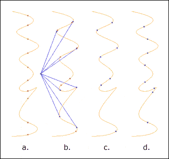
• 1st Image: Intersection of a curve with an infinite plane
• 2nd Image: 3D Silhouette Computation (perspective - blue, parallel projection - red)
• 3rd Image: Points on curve where tangent is parallel to a given vector
• 4th Image: Inflection points of a curve - points with zero curvature

Figure 6: Curve Properties and Analysis continued

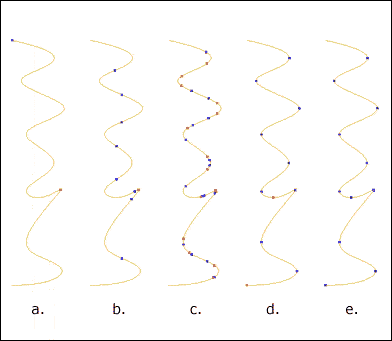
• 1st Image: Minimum (red) and maximum (blue) first derivative magnitudes
• 2nd Image: Minimum (red) and maximum (blue) radius of curvature
• 3rd Image: Find first derivative (blue) and radius of curvature(red) of given magnitude
• 4th Image: Find points on curve where first derivative is perpendicular to a given axis (blue - X axis, red - Y axis)
• 5th Image: Find points on a curve where first derivative is perpendicular to any axis

Composite Curve ( IwCompositeCurve)

• Creation of composite curves from an unordered set of curves
• Offset of a composite curve with filleting or extension and trimming - see Figure 13
• Simultaneous offset of multiple composite curve loops (i.e. face with holes)
• Creation of a single NURBS curve from a composite

Figure 13: Offsetting/Insetting Composite Curves

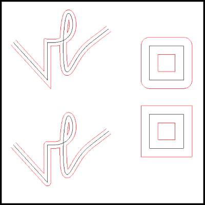
Shown are linear extension and corner filleting.

B-Spline Curve (IwBSplineCurve)

• construction/editing/query using STEP format or NLib data structures
• continuity calculation, removal of extra knots, conversion to 2D
• creation by joining connected curve segments
• creation of a circle segment, ellipse segment line segment, degenerate curve
• creation of mirror curve
• editing the end points of a B-Spline
• extraction of analytical information for lines and arcs
• offseting of smooth curves

Curve/Point - see Figure 1

• minimization - find point(s) on curve closest to the point
• maximization - find point(s) on curve farthest from the point
• normalization - find point(s) on curve where tangent is perpendicular to vector to the point
• at distance - find point on curve at given distance from point
• intersection - find parametric value(s) on curve corresponding to the point
• projected minimization and maximization - as projected to a plane
• directed minimization and maximization - along a vector as projected to a plane

Figure 1: Curve/Point Solver

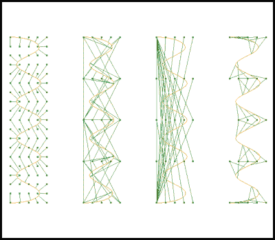
• 1st Image - Minimization of a point and curve. Finds the closest point between a curve and a point. Note that some points have multiple closest points because of curve symmetry.
• 2nd Image - Normalization of point and curve. Finds position on a curve where vector from a point to a curve is perpendicular to the curve's tangent vector.
• 3rd Image - Maximization of point and curve. Finds the farthest point between a curve and a point.
• 4th Image - At Distance between of point and curve. Finds the position on a curve at a given distance from a point.

Curve/Curve - see Figure 2

• minimization - find points on the two curves where the distance between them is minimal
• maximization - find points on the two curves where the distance between them is maximal
• normalization - find points on the curves where the tangents are perpendicular to the vector between the curves
• at distance - find points on the two curves which have a given distance between them and have the same angle to the vector between them
• projected solvers - intersection, minimization, maximization, directed minimization, signed directed minimization, angle to plane, angle between, signed pivot angle between
• 3D directed minimization - collision detection - find first contact point moving along a 3D vector

Figure 2: Curve/Curve Solver

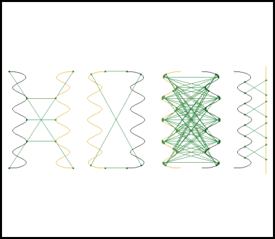
• 1st and 2nd Image: Minimization and maximization of two symmetric nurbs. Note that multiple answers result when more than one minimum or maximum points fall within the user specified tolerance.
• 3rd Image: Normalization between two curves finds all points where the vector between two points is perpendicular to the tangent vectors of the curves at those points.
• 4th Image: At Distance between two curves finds corresponding points on two curves which are at a given distance and the angle between the tangent vectors are equivalent.

3D Curve/Curve Intersection - see Figure 3

• handles coincidence, tangency, near tangency, and grazing conditions
• projected curve/curve intersection
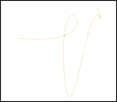
• self-intersection detection is also provided - See Figure 4

Figure 3: Curve/Curve Intersection - produces either single points or coincident segments (3rd Image)

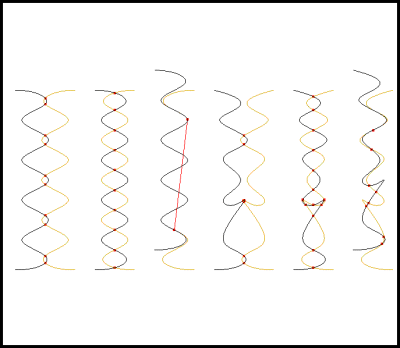
Figure 4: Curve self-intersection - finds points where the curve crosses itself

Surface (IwSurface)

• point and derivative evaluation, evaluation of geometric properties
• normal evaluation, evaluation of a normal section
• high precision surface area computation
• dropping 3D vectors into parameter space
• closed and periodic testing, singularity testing
• validation
• transformation

B-Spline Surface ( IwBSplineSurface )

• construction using STEP format or NLib data structures
• continuity calculation
• query
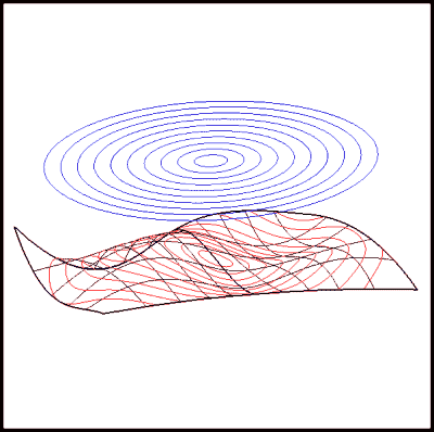
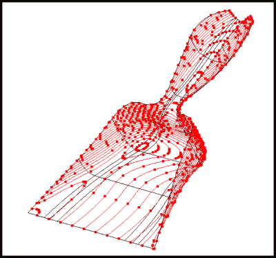
• creation of planar section curves - see Figure 14
• creation of parallel projection curves - see Figure 15

Figure 14: Creation of Planar Section Curves

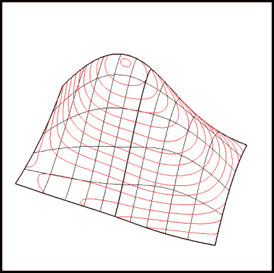
Figure 15: Creation of Curves by Parallel Projection

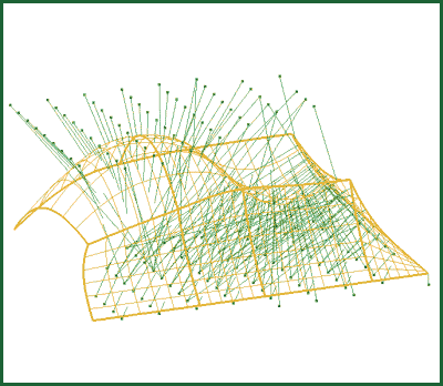
Surface/Point - see Figure 7 and Figure 8

• minimization - find point(s) on surface closest to point
• maximization - find point(s) on surface farthest from the point
• normalization - find point(s) on surface where normal is parallel to vector to point
• intersection - find parametric value(s) on surface corresponding to the point
• 3D directed minimization - collision detection - find first contact point moving along a 3D vector

Figure 7: Surface/Point Solver - minimization (closest point) between a point and a surface

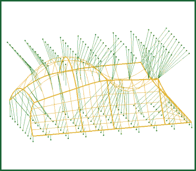
Figure 8: Surface/Point Solver - normalization of a point and a surface

Surface/Curve - see Figure 9

• minimization - finds where distance between curve and surface is minimal
• maximization - finds where distance between curve and surface is maximal
• normalization - finds where vector between entities is parallel to surface normal and perpendicular to the curve tangent
• 3D directed minimization - collision detection - find first contact point moving along a 3D vector

Figure 9: Surface/Curve Solver

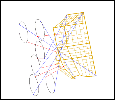
Minimization (red) and maximization (blue) of the distance between a curve and a surface.

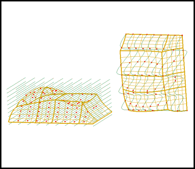
Curve/Surface Intersection - see Figure 10

• handles coincidence, tangency, near tangency, and grazing conditions.

Figure 10: Curve/Surface Intersection

Surface/Surface - see Figure 11

Local and global version of the following:

• minimization - find where distance between surfaces is minimal
• maximization - find where distance between surfaces is maximal
• normalization - finds where vector between surfaces is parallel to surface normals
• 3D directed minimization - collision detection - find first contact point moving along a 3D vector

Figure 11: Surface/Surface Solver

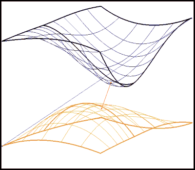
minimization (red) and maximization of the distance between two surfaces.

Dropping Curves - see Figure 12

• create the 2D parameter space curve(s) corresponding to a 3D curve which lies on or near a surface
• restricted to surfaces with at least C1 continuity
• advanced dropping which allows C0 continuity surfaces

Figure 12: Dropping Curves

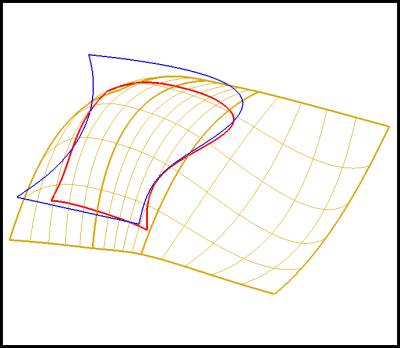
Produce a 2D parameter space image of a 3D curve.

Numerical utility classes

• IwIntegrator - provides numerical integration
• IwLocalSolve1d - provides one-dimensional Newton based local solver algorithm
• IwLocalSolveNd - provides N-dimensional Newton based local solver algorithm
• IwGlobalSolver - provides global solver algorithms

Advanced Surfaces

Advanced Surface/Surface Intersection - see Figure 16

Figure 16: Surface/Surface Intersection with curve knots displayed

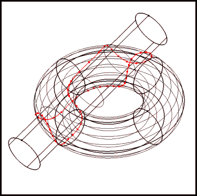
• Extension of basic surface/surface intersection found in GSLib
• Adds the ability to extract intersection curves along surface tangencies - surface normals are parallel along the intersection curve - see Figure 22
• Adds the ability to process curves where singularities occur - point where surface normal are parallel and intersection curves pass through the point - see Figure 23
• Adds the ability to produce zero length or NULL curves - point where surfaces touch at a single point but do not intersect near that point - see Figure 24
• Fast detection of interior closed intersection loops - see Figure 25
• Enhances the performance of the basic intersector

Figure 22: Surface/Surface Intersection with Tangent Surfaces

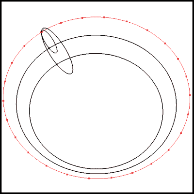
Figure 23: Surface/Surface Intersection with Singularity Points

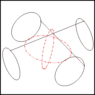
Figure 24: Surface/Surface Intersection

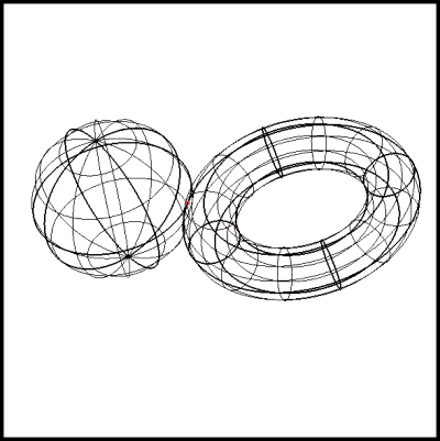
which produces a zero length curve.

Figure 25: Surface/Surface Intersection

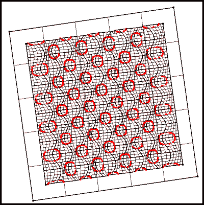
which produces multiple intersection loops.

Surface Curve Tracing Abstract Class (IwSurfaceTracer)

• Provides an Object-Oriented Framework which should enable the fast implementation of additional curve extraction utilities through subclassing and implementation of virtual methods.

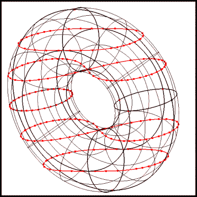
Sectioning of a Surface with an Infinite Plane (IwSurfaceSection) - see Figure 26
Figure 26: Surface Sectioning with a Plane

• Implementation in context of the Curve Tracing Framework.
• Able to detect curves where surface is tangent to the plane.
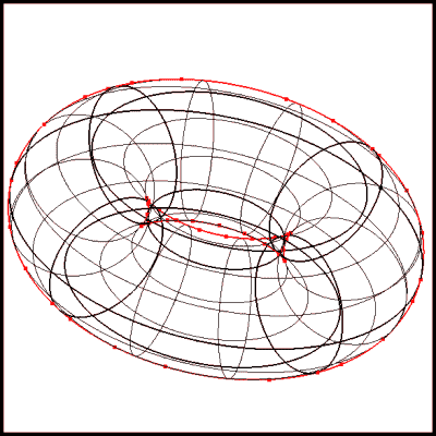
• Able to detect singularity points (points where 4 curves come to a point) - see Figure 27
• Able to detect tangent points (point where surface touches plane at a single point) - see Figure 27

Figure 27: Surface Sectioning with a Plane

Surface Silhouette Curve Creation (IwSurfaceSilhouette) - see Figure 17

• Implementation in context of the Curve Tracing Framework.
• Able to detect all silhouette curves on a surface - see Figure 29
• Able to detect silhouettes which correspond to iso-parametric curves.
• Able to detect silhouettes which pass through the poles of the surface.

Figure 17: Surface Silhouette Curve Extraction

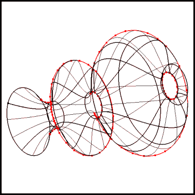
Figure 29: Surface Silhouette Curve Extraction

Curve Projection on C0 Surfaces (IwSurfaceDropCurve)

• Provides for the creation of UV trim curves from 3D curves
• Surfaces may have discontinuities of the tangent plane (C0 continuity)
• Requires that the 3D curve lie on or very close to the surface