Infrastructure Scaling

We benchmarked Kumo Engine 1.0.0 on one AWS g6e.8xlarge with a single NVIDIA L40S GPU to understand how database structure and size affect a complete training and prediction workflow. We measured source staging, graph creation, training-table generation, fit, and prediction while varying table count, relationship layout, row volume, and feature width.

Adding tables increased runtime across the measured schema families, but the relationships between those tables changed how much work followed. At 64 tables, the chain took 335.2 seconds across stages, compared with 477.4 seconds for the star and 498.9 seconds for the mapping schema. Most of that difference was in fit. The examples below show how the same five tables can form each layout.

Chain: T4 links through T3, T2, and T1 to prediction entity T0.

Tree: T1 and T2 link to prediction entity T0, while T3 and T4 link to T1.

Mapping: T2, T3, and T4 each link to prediction entity T0 and second parent T1.

Cycle: a chain of five tables closes with a relationship from T0 back to T4.

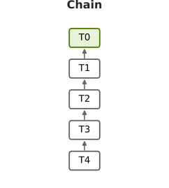
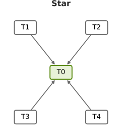
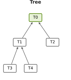
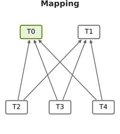
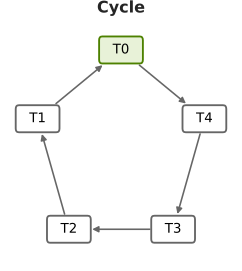
These five-table examples illustrate the relationship layouts. T0, shaded green, is the prediction entity. Each arrow points from a child’s foreign key to its parent’s primary key.

Row growth and feature growth affected different parts of the workflow. In the three-table row sweep, increasing the mapping table from 10 million to 100 million rows raised graph-build time from 29.7 to 83.0 seconds, while fit stayed near 116 to 118 seconds. At a fixed 10 million mapping rows, widening that table from 2 to 500 columns increased fit from 75.7 to 923.1 seconds.

For users planning work on a large database, these results suggest three priorities:

Pilot the actual schema and prediction target. Preserve important relationships and mapping tables. Table count alone did not rank runtime.
Plan preparation and model execution separately. More rows can add substantial staging and graph-build work even when the training budget stays fixed. Include case overhead in job-duration estimates.
Review feature width and measure resource use. Wider tables increased both fit and prediction time. Evaluate which features the task needs, and measure system RAM and local scratch alongside compressed source bytes before sizing the full graph.

Timing measures and stages

All results on this page use g6e.8xlarge measurements. Main tables and plots show the first measured run of each workload. Case wall captures the elapsed workflow; stage sum adds its five timed operations.

Stage or measure	Timed operation
Case wall	Elapsed time from the runner’s recorded start to completion, including setup, all five stages, validation, and local model/prediction copying
Stage sum	Sum of source staging, graph build, training-table creation, fit, and prediction
Source staging	Read source manifests and download source Parquet from S3 to local storage
Graph build	Create the graph snapshot and its indexes from the staged source
Training table	Generate the query’s training table and split
Fit	Execute the fit call, including setup, sampling, training, and evaluation
Predict	Create the prediction-table object and predict for 8,192 entities

Case wall time split into the five measured stages and other case overhead, comparing five 64-table schemas and five three-table mapping-row volumes.

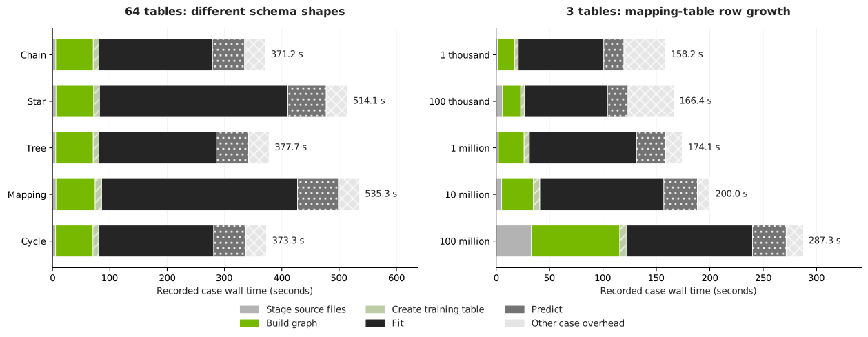
Each complete bar is case wall time. The pale hatched segment is case overhead outside the five stages.

The 64-table chain took 371.2 seconds of case wall time, including 335.2 seconds across stages and 36.1 seconds of other case overhead. The mapping schema took 535.3 seconds of case wall time and 498.9 seconds across stages.

Stage timings at 64 tables

Schema	Case wall s	Stage sum s	Staging s	Graph s	Training table s	Fit s	Predict s
Chain	371.2	335.2	5.8	65.3	9.9	198.1	56.1
Star	514.1	477.4	6.1	65.8	10.0	328.6	66.9
Tree	377.7	341.8	5.7	65.3	9.8	204.7	56.3
Mapping	535.3	498.9	6.1	68.3	11.3	341.7	71.4
Cycle	373.3	336.9	5.5	65.2	9.8	200.7	55.7

Times are seconds, rounded independently to one decimal place. Displayed stages can therefore differ slightly from the displayed sum. Unrounded values are available in the raw run table and individual stage records.

Schema and table-count scaling

Each table in this experiment contains 100,000 rows and 32 columns. Adding tables therefore increases the source volume as well as changing the graph. The layouts shown above connect those tables in different ways.

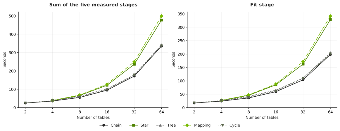
Total stage time and fit time versus table count for chain, star, tree, mapping, and cycle schemas.

Lines connect measured workloads. The left panel shows stage sum; the right shows fit. Both use the same table-count axis.

The table reports stage sums for every measured schema and table count. The source column gives the chain’s total compressed Parquet size as a reference. Other schemas have similar source sizes; their exact values are in the downloads.

Tables	Chain source GB	Chain s	Star s	Tree s	Mapping s	Cycle s
2	0.016	25.0	Not run	Not run	Not run	25.6
4	0.032	35.9	38.3	37.9	39.3	38.0
8	0.065	55.6	66.6	62.4	68.7	58.4
16	0.131	95.0	122.1	102.1	127.7	97.3
32	0.263	172.0	236.3	178.4	250.1	178.5
64	0.527	335.2	477.4	341.8	498.9	336.9

The two-table star and tree are equivalent to the two-table chain and were not run separately. The mapping experiment starts at four tables.

Chain

Each successive table links to the preceding table. Increasing from 2 to 64 tables raised stage sum from 25.0 to 335.2 seconds (13.4 times), while compressed source size grew 33.5 times. From 32 to 64 tables, stage sum grew from 172.0 to 335.2 seconds, or 1.95 times. Fit accounted for 198.1 seconds at 64 tables.

Star

Every child table links to the central prediction entity. At 64 tables, star and chain use the same source tables and 0.527 GB of Parquet, each with 63 declared relationships. Star’s stage sum was 42.4% longer than chain’s, while graph build was nearly unchanged at 65.8 versus 65.3 seconds.

Fit increased from 198.1 seconds for chain to 328.6 seconds for star, accounting for about 92% of the additional stage time. Within the star family, moving from 32 to 64 tables increased stage sum from 236.3 to 477.4 seconds, or 2.02 times.

Tree

Tables form a binary branching hierarchy. Stage sum grew from 37.9 seconds at four tables to 341.8 seconds at 64 tables. The 64-table tree uses the same source tables and relationship count as the chain and star. Its 204.7-second fit and 341.8-second stage sum stayed close to the chain’s 198.1 and 335.2 seconds.

Mapping

Each mapping table links to two entity/metadata parents. Stage sum grew from 39.3 seconds at four tables to 498.9 seconds at 64 tables. At 64 tables, the schema has 124 declared relationships, compared with 63 for the chain, and uses different table roles.

Its stage sum was 48.8% longer than the chain’s, with fit increasing from 198.1 to 341.7 seconds. From 32 to 64 tables, mapping stage sum grew from 250.1 to 498.9 seconds, or 1.99 times.

Cycle

A closing relationship connects the ends of a chain. Stage sum grew from 25.6 seconds at two tables to 336.9 seconds at 64 tables. At 64 tables, graph build took 65.2 seconds and fit took 200.7 seconds, close to the chain’s 65.3 and 198.1 seconds in this experiment.

Together, the matched chain, star, and tree results show why relationship layout belongs in a sizing pilot. Their source bytes and relationship counts match, yet their fit times differ. That is consistent with different sampling and model execution work around the prediction entity; the stage timings do not isolate the individual operations responsible inside fit.

Row-volume scaling

This experiment holds the schema at three tables. Two parent tables each contain 1 million rows and 32 columns. The mapping table also has 32 columns, and only its row count changes. Even the smallest case therefore contains more than 2 million total source rows.

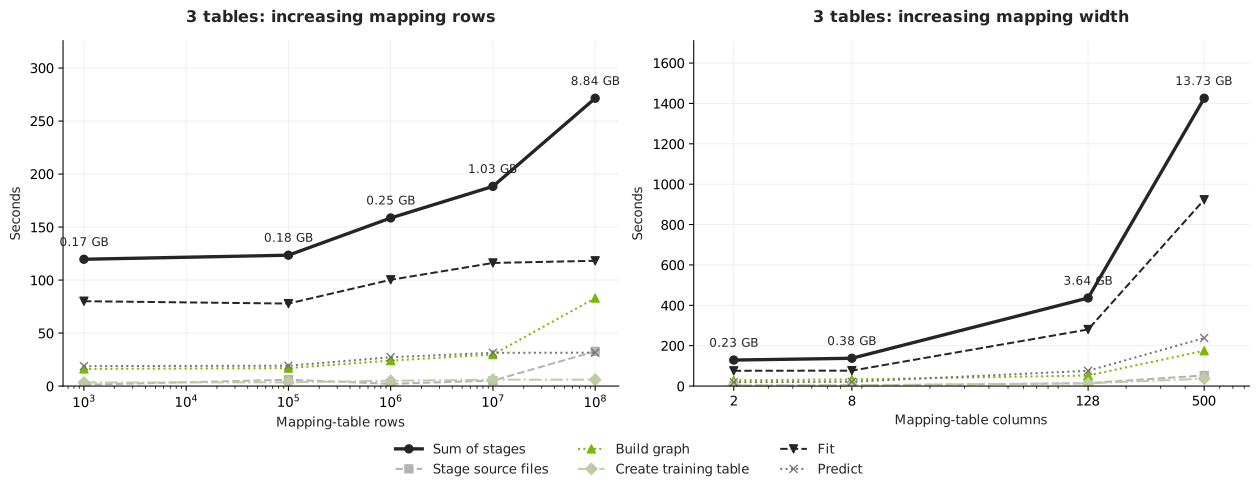
Stage times versus mapping-table row count and column count, with total compressed source GB annotated at each measured point.

The left panel varies mapping rows with 32 columns. The right varies mapping columns with 10 million rows. Both contain three tables, and the y-axis scales differ.

Mapping rows	Source GB	Case wall s	Stage sum s	Staging s	Graph s	Training table s	Fit s	Predict s
1,000	0.167	158.2	119.6	1.2	16.2	3.4	80.1	18.8
100,000	0.175	166.4	123.5	6.0	17.0	3.5	77.8	19.2
1,000,000	0.254	174.1	158.6	2.1	24.0	5.0	100.2	27.2
10,000,000	1.034	200.0	188.4	5.2	29.7	6.0	116.1	31.4
100,000,000	8.843	287.3	271.5	32.7	83.0	6.1	118.2	31.5

From 1 million to 100 million mapping rows, total source size increased from 0.254 to 8.843 GB, about 34.9 times. Stage sum increased 1.71 times, from 158.6 to 271.5 seconds. Graph build rose from 24.0 to 83.0 seconds, while fit rose from 100.2 to 118.2 seconds.

The upper interval shows where the added work went. From 10 million to 100 million mapping rows, source bytes increased 8.55 times. Staging grew from 5.2 to 32.7 seconds and graph build from 29.7 to 83.0 seconds. Fit changed from 116.1 to 118.2 seconds, and prediction from 31.4 to 31.5 seconds, under the same training budget and prediction cohort.

Feature-width scaling

The mapping table stays at 10 million rows while its total column count grows. Both parent tables keep their rows and 32-column widths. Width 2 means a mapping table with only two foreign-key columns. Wider mapping tables add a primary key and feature columns, so the first transition includes a structural change.

Mapping columns	Source GB	Case wall s	Stage sum s	Staging s	Graph s	Training table s	Fit s	Predict s
2	0.233	139.5	128.9	2.2	28.6	3.3	75.7	19.0
8	0.383	151.6	137.8	2.6	33.0	4.4	76.5	21.3
128	3.639	453.8	436.4	14.6	52.3	13.5	280.3	75.6
500	13.730	1452.6	1425.7	52.7	175.1	36.7	923.1	238.1

From 2 to 500 mapping columns, stage sum increased 11.1 times, from 128.9 to 1,425.7 seconds. Fit increased 12.2 times, from 75.7 to 923.1 seconds, and prediction increased 12.5 times, from 19.0 to 238.1 seconds. The widest case took 1,452.6 seconds (24.2 minutes) of case wall time.

Feature growth increased model execution time substantially even with the same optimizer-step and prediction-count limits. Fit accounted for about 65% of the widest case’s stage sum. Reviewing relevant features can therefore matter alongside planning for more rows. Evaluate held-out quality before excluding columns or changing sampling settings.

Memory and storage planning

Two additional three-table workloads illustrate why source bytes alone do not rank resource demand. A compact billion-row mapping table used more sampled system memory than a substantially larger, wider source:

Three-table workload	Mapping rows / columns	Source GB	Case wall s	Stage sum s	System memory GiB	Scratch growth GiB
Compact mapping	1,000,000,000 / 2	6.816	317.4	304.7	116.69	63.37
Wide mapping	38,999,332 / 500	53.062	1970.8	1939.9	66.86	218.30

These are separate workloads. The compact mapping table has two columns and the wide mapping table has 500. System memory is the sampled physical memory in use; scratch growth is the increase in used space on the scratch filesystem.

Use the GPU sizing guide when provisioning: allow at least 4 times source size in free local SSD scratch, or 8 times for graphs with many edges. Recommended RAM meets both 4 GiB per vCPU and 1.5 times source size. Allow additional space for staged source files and retained snapshots or outputs on the same filesystem, then verify actual use with a representative pilot.

Methodology

The methodology focused solely on infrastructure benchmarking: elapsed time, system memory, and local scratch use. Predictive accuracy was outside the evaluation.

Hardware capacities are from AWS’s G6e specifications. Each run used a fresh graph scratch directory, and filesystem caches were dropped before graph creation. The loader settings below are benchmark controls rather than recommended defaults for every workload.

Setting	Value
Engine and measurement date	Kumo Engine 1.0.0; November 4, 2026 (UTC)
Compute	g6e.8xlarge; 32 vCPUs; 256 GiB system RAM
Accelerator	One NVIDIA L40S; 48 GB nominal GPU memory
Working storage	Local NVMe instance store; 900 GB nominal capacity
Source data	Synthetic relational Parquet with numeric, categorical, and temporal columns
Prediction task	Binary classification on the designated entity table
Training budget	200 optimizer steps: two epochs capped at 100 steps each; batch size 256
Model and sampling	GNN with 64 channels; two sampling hops, with defaults of 10 and 5 neighbors
Evaluation	Random 80/10/10 split; validation and test capped at 20 steps per pass
Prediction cohort	8,192 entities per run
Data loader	Eight workers, standalone mode, two Rayon threads

Experiment	What changes	What stays fixed
Schema and table count	Table count and relationship layout	100,000 rows per table; 32 columns per table
Row volume	Mapping-table rows	Three tables; 32 columns each; two parent tables of 1 million rows each
Feature width	Mapping-table columns	Three tables; 10 million mapping rows; two parent tables of 1 million rows and 32 columns each

Source sizes sum all tables’ compressed Parquet bytes and use decimal GB (1 GB = 1 billion bytes). Memory and scratch use GiB (1 GiB = 1,073,741,824 bytes).

Repeatability

Two anchor workloads were run three times:

Case	Metric	Runs	Median s	Observed range s
`star-16`	Stage sum	3	122.07	122.05 to 122.78
`star-16`	Case wall	3	139.19	138.90 to 141.00
`rows-10000000`	Stage sum	3	189.20	188.39 to 189.49
`rows-10000000`	Case wall	3	202.19	200.02 to 202.99

These ranges describe the anchors. Other workloads have one baseline run, so small differences should not be treated as established rankings. Main tables and plots consistently retain the first run rather than mixing it with repeat medians.

Next steps and limits

The table-count experiment grows total rows and source bytes as it adds tables. The controlled row-volume sweep exists only at three tables. There is no measured volume sweep within the 4-, 8-, 16-, 32-, or 64-table schemas. The 64-table graphs contain about 0.527 GB of source Parquet; these runs do not establish capacity or runtime for large 64-table databases.

The row-volume experiment fixes optimizer steps and prediction rows. Larger training budgets, model plans, or prediction cohorts need separate measurements. The memory sampler ran every two seconds, so shorter peaks may be missed. Observed resource peaks are not minimum safe provisioned capacities.

For your next evaluation, preserve the intended query, relationship structure, feature widths, and representative key distributions. Measure progressively larger row volumes within that schema. Record case wall time, individual stages, system RAM, GPU memory, and scratch use, then choose capacity and training settings from those measurements. The Model Plan Guide explains the settings to record and control.

Download measurements

The tables above cover 27 topology workloads, five row-volume workloads, and four width workloads. The downloads include all 48 measured g6e.8xlarge baseline runs across 44 distinct workloads, including encoding and stress experiments and four additional anchor repetitions.

Raw run table (CSV)

Individual stage records (CSV)

Both tables with a column guide (ZIP)