Temporal Hetero-GNN | NVIDIA Kumo

Kumo Engine’s built-in model is a temporal heterogeneous graph neural network (hetero-GNN) for relational data. It follows the relational deep learning formulation of Fey et al. (2024): each table row is a node, each primary key/foreign key link is a typed edge, and each prediction is computed from a subgraph sampled around the target entity, using only rows from before the prediction time. The same architecture handles classification, regression, forecasting, and link prediction.

It combines ideas from several papers, including GraphSAGE’s neighbor sampling, R-GCN’s relation-specific weights, PNA’s multiple aggregators, and the ID-GNN and ContextGNN models for link prediction. The combined architecture has been tested on hundreds of datasets and runs in production at many organizations.

Supported Task Types

Kumo reads the task from the predictive query, including its target, labels, and time horizon, and attaches the matching prediction head and loss.

Task	Output	Example
Binary and multiclass classification	Class probabilities for each entity	Whether a transaction is fraudulent
Multilabel classification	A probability for each label	Which categories a customer will buy from
Multilabel ranking	Labels in score order	A customer’s interests, ranked
Regression	One number for each entity	A customer’s spend over the next month
Forecasting	One number for each future time window	Daily demand over the next week
Static link prediction	A score for each candidate link	User-product links missing from the data
Temporal link prediction	A score for each candidate future interaction	The products a customer will buy next

Classification, regression, and forecasting are node tasks, where the output belongs to the entity at the root of the sampled subgraph. Link prediction scores pairs of a source entity and a candidate target. Both kinds can be temporal, in which case each training example has a prediction time, with inputs from rows before it and labels from the horizon after it. Static link prediction instead holds out a random subset of existing links for evaluation.

See Predictive Queries.

Feature Encoders

Before message passing, each row is encoded into a fixed-width vector that becomes its node’s initial representation. Encoders are defined per table and, within a table, per column. Kumo picks each column’s encoder from its semantic type (stype) and statistics, then combines the column outputs. This per-stype design comes from PyTorch Frame (Hu et al., 2024).

Column stype	Encoders
Numerical	`Numerical` rescales the value. `MaxLogNumerical` and `MinLogNumerical` compress heavy tails with a log transform.
Categorical, ID	`Index` learns one vector per category. `Hash` maps categories into a fixed number of buckets, bounding memory at the cost of collisions.
Multicategorical	`MultiCategorical` combines the vectors of every category in a cell.
Text	`TextEmbedding` averages pretrained word vectors.
Timestamp	`Datetime` encodes calendar components: minute, hour, day of week, day of month, day of year, and year.
Numerical vector	`NumericalList` takes fixed-length vectors, including embeddings computed outside Kumo.

Null excludes a column from the features. A key column excluded this way still defines its edges in the graph. See Encoder Selection.

Each sampled row is also encoded with the time between its timestamp and the prediction time, which lets the model tell a purchase made ten minutes before a transaction from one made a year earlier. use_seq_id optionally adds the order of the sampled events, and prediction_time_encodings adds the absolute prediction time.

Model Architectures

Heterogeneous GNN

The GNN runs on a subgraph sampled around the target entity with a fixed fanout per hop, as in GraphSAGE (Hamilton et al., 2017). Fanouts can be overridden per edge type, and adaptive sampling shifts budget to later hops when earlier hops come up short.

Each table is a node type, and each foreign key defines an edge type in each direction. The GNN learns separate weights for every edge type, the construction introduced by R-GCN (Schlichtkrull et al., 2018) and provided in PyG by HeteroConv and to_hetero (Fey and Lenssen, 2019).

On the one side of a one-to-many relationship, a node aggregates many neighbors, as an account does with its transactions. Following PNA (Corso et al., 2020), Kumo combines several aggregators, such as sum, mean, and max, because each loses different information: mean discards neighborhood size, which sum preserves (Xu et al., 2019), and max keeps only the extreme. On the many side, each row receives the representation of the single row it references. A learned skip connection carries each node’s own representation into the next layer.

Schematically, for a prediction at time $t$ , one layer updates a node $v$ of type $\tau(v)$ as

h_v^{(\ell+1)} = \sigma\Big( W_{\tau(v)}^{(\ell)}\, h_v^{(\ell)} \;+ \sum_{r \in \mathcal{R}(v)} \operatorname{AGG}_r \big\{ W_r^{(\ell)}\, h_u^{(\ell)} \;:\; u \in \mathcal{N}_r^{t}(v) \big\} \Big)

where $\mathcal{R}(v)$ is the set of edge types that end at $v$ ‘s table, $\mathcal{N}_r^{t}(v)$ is the set of $v$ ‘s sampled neighbors under edge type $r$ that are visible at time $t$ , and $\operatorname{AGG}_r$ combines the configured aggregators. Normalization, dropout, and the MLP layers before and after message passing are omitted.

Each layer extends the receptive field by one hop, and the number of layers equals the sampling depth. For a transaction $v$ scored for fraud, the first hop reaches its account $a$ and its merchant $m$ , and the second reaches the account’s earlier transactions and the merchant’s other transactions.

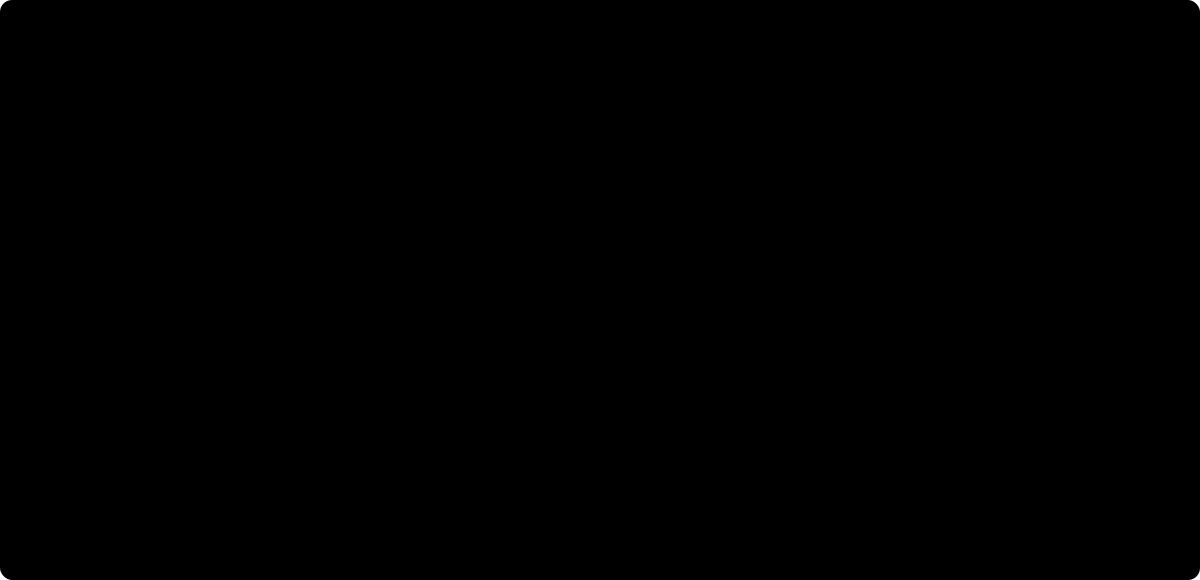
A two-hop temporal subgraph for a transaction scored at time t, and two layers of message passing over it.

The remaining layer choices follow the GNN design space of GraphGym (You et al., 2020): MLP layers before and after message passing, activation, normalization, and dropout. The model plan can search over these along with hidden width and the aggregator set.

Graph Transformer

GraphTransformerModelPlan replaces hop-by-hop message passing with self-attention over every node in the sampled subgraph, letting any two sampled rows exchange information in one layer rather than through the nodes between them. Since attention ignores graph structure, each node also gets positional encodings. hop embeds the node’s distance from the target entity. random_gnn adds the output of a small GNN run over random initial features, which captures the node’s local structure. These correspond to the hop-distance and subgraph-GNN encodings in the Relational Graph Transformer (Dwivedi et al., 2026), and the use of random features to break symmetry between otherwise identical nodes goes back to Sato et al. (2021).

Unlike the GNN’s, the transformer’s depth is not tied to sampling depth; you set the number of layers and attention heads separately. It supports node tasks, including forecasting, but not link prediction. See Relational Graph Transformers.

Identity-Aware Message Passing

Without distinguishing node features, a standard GNN cannot tell a node in a triangle from a node in a square, because their computation trees are identical. ID-GNN (You et al., 2021) colors the node being embedded wherever it recurs in its own tree and gives messages from colored nodes separate weights, which makes the trees distinguishable. For link prediction, the source node is colored instead, so a candidate’s representation depends on how it connects to that source. The "pairwise" and "context" link prediction modules are built on this.

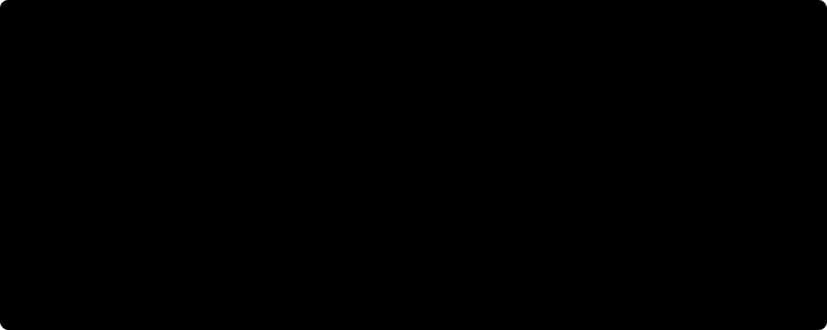
Node v1 sits in a triangle and node v2 in a square. A standard GNN produces identical three-layer computation trees for both. ID-GNN colors the root wherever it recurs: in v1's tree it recurs at depths 2 and 3, in v2's tree only at depth 2, so the trees and the representations differ.

After You et al. (2021), Figure 1. Nodes have no distinguishing features.

Kumo applies the same idea when a classification or regression query involves several entities: it marks each entity’s role and combines their representations in a joint prediction head.

Link Prediction Variants

The main design choice in link prediction is how to represent candidate targets. A two-tower model embeds sources and targets independently and ranks pairs by similarity. Target embeddings can then be computed once, which scales to large catalogs, but a target looks the same to every source. A pair-wise model such as ID-GNN conditions each target on the source at the cost of one representation per pair, which in practice limits it to candidates inside the source’s sampled subgraph. ContextGNN (Yuan et al., 2025) fuses the two, using pair-wise scores for candidates near the source and two-tower scores for the rest.

plan.model_architecture.module selects among these:

Module	Architecture	Task support
`"shallow_rhs"`	A GNN representation of the source is scored against a shallow embedding of each target, which is learned per target, built from its encoded columns, or both. This has the same form as ContextGNN’s two-tower component.	Static and temporal
`"two_tower"`	The GNN encodes the source’s and the target’s neighborhoods separately and ranks pairs by embedding similarity.	Static and temporal
`"pairwise"`	ID-GNN. Message passing conditioned on the source scores each candidate in the source’s sampled subgraph.	Temporal
`"context"`	ContextGNN. `"pairwise"` scores for candidates in the sampled subgraph are fused with `"shallow_rhs"` scores over the full candidate set.	Temporal

For "shallow_rhs" and "context", target_embedding_mode sets how target embeddings are built, and with it whether the model can score targets that were not in the training data. "lookup" learns a free vector per training target and cannot score new ones. "feature" and "shallow_feature" derive the vector from the target’s encoded columns, "feature" through a deeper learned projection and "shallow_feature" through normalization alone. "fusion" adds the lookup and feature vectors. To score new targets, use a feature mode and set handle_new_target_entities=True.

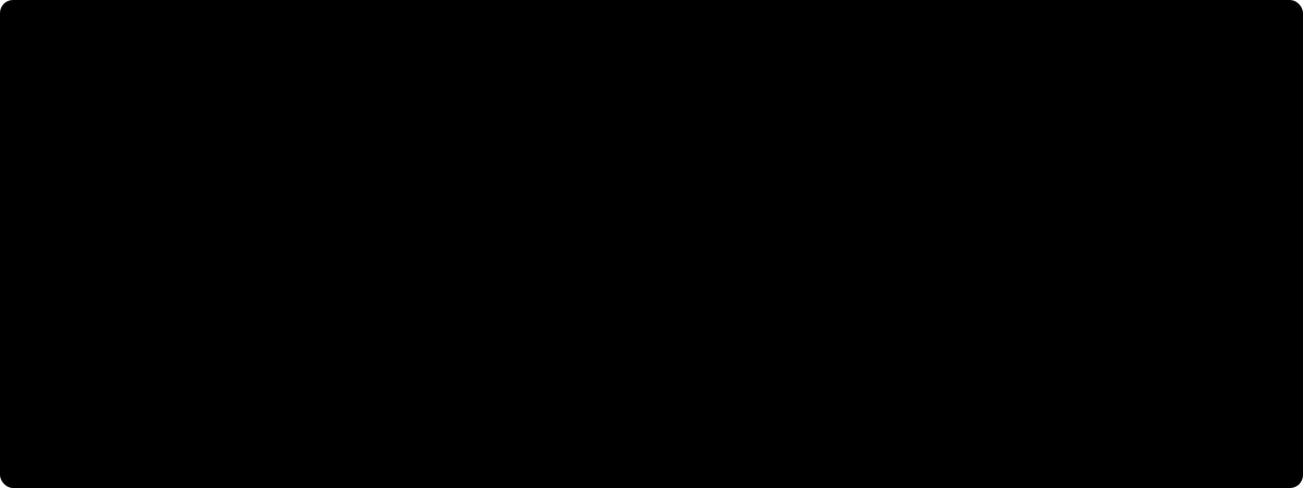
Entity tower: a heterogeneous GNN aggregates the source customer's transactions and their products into a vector h_c. Target tower: each product's vector e_p is the sum of an MLP over its features and its row in a lookup table, with no message passing. A dot product of h_c and e_p feeds a softmax over products.

"shallow_rhs" with target_embedding_mode="fusion".

For learned embeddings, we recommend "shallow_rhs" with hybrid lookup and feature embeddings. "two_tower" is fully inductive: it computes both source and target embeddings from their features and graph neighborhoods.

See Link Prediction and Embeddings, Product Recommendations, and Hybrid GNNs for Recommendations.

Forecasting Variants

The forecasting head combines the entity’s graph representation with the target’s own recent history, taken from the lag windows generated with the training table. past_encoder selects how that history is encoded: "decomposed" (the suggested default), "normalized", "mlp", or "transformer". A separate encoder handles previous-year values when the training table includes them. The head is either shared across entities, which lets it forecast for entities absent from training (handle_new_entities=True), or extended with learned parameters for each training entity (False).

See Forecasting Architecture and Historical Inputs and Time Series Forecasting.

Putting It Together

The model plan defines the architecture search space. Kumo Engine automatically runs hyperparameter search using Optuna’s Tree-structured Parzen Estimator (TPE). To define your search space, list the options you want to try for each parameter.

Here’s an example using the query, training_table, and snapshot from Getting Started:

from kumo.engine import Trainer
from kumoapi.model_plan import GNNModelPlan
plan = query.suggest_model_plan(snapshot)
plan.model_architecture.model = [GNNModelPlan(
    channels=[64, 128],
    aggregation=[["sum", "mean", "max"], ["mean"]],
    dropout=[0.0, 0.1],
)]
plan.neighbor_sampling.num_neighbors = [[20, 10], [20, 10, 5]]

The sampling configuration also sets the GNN depth: [20, 10] gives two message-passing layers, while [20, 10, 5] gives three.

Next, set a budget of eight trials, each with up to 20 training epochs, and train:

plan.training_job.num_experiments = 8
plan.optimization.max_epochs = 20
trainer = Trainer(plan)
result = trainer.fit(training_table, snapshot=snapshot)
print(result.metrics)

The fitted trainer holds the model selected by validation performance. Use it to save predictions and customer embeddings as Parquet. Choose a new output directory for each run:

from kumo.engine import FileConnector, PredictionOutputConfig
prediction_table = query.generate_prediction_table(snapshot)
predictions = trainer.predict(
    prediction_table,
    snapshot=snapshot,
    binary_classification_threshold=0.5,
    output_config=PredictionOutputConfig(
        connector=FileConnector(root_dir="./results/run-001"),
        output_paths={
            "predictions": "predictions/",
            "embeddings": "embeddings/",
        },
    ),
)
print(predictions.frame.head())

See the Model Plan Guide, Making Predictions, and Generate and Save Embeddings.

References

Corso, G., et al. “Principal Neighbourhood Aggregation for Graph Nets.” NeurIPS 2020. arXiv:2004.05718
Dwivedi, V. P., et al. “Relational Graph Transformer.” ICLR 2026. arXiv:2505.10960
Fey, M., and Lenssen, J. E. “Fast Graph Representation Learning with PyTorch Geometric.” ICLR Workshop on Representation Learning on Graphs and Manifolds, 2019. arXiv:1903.02428
Fey, M., et al. “Relational Deep Learning: Graph Representation Learning on Relational Databases.” ICML 2024. arXiv:2312.04615
Hamilton, W. L., Ying, R., and Leskovec, J. “Inductive Representation Learning on Large Graphs.” NeurIPS 2017. arXiv:1706.02216
Hu, W., et al. “PyTorch Frame: A Modular Framework for Multi-Modal Tabular Learning.” 2024. arXiv:2404.00776
Sato, R., Yamada, M., and Kashima, H. “Random Features Strengthen Graph Neural Networks.” SDM 2021. arXiv:2002.03155
Schlichtkrull, M., et al. “Modeling Relational Data with Graph Convolutional Networks.” ESWC 2018. arXiv:1703.06103
Xu, K., Hu, W., Leskovec, J., and Jegelka, S. “How Powerful are Graph Neural Networks?” ICLR 2019. arXiv:1810.00826
You, J., Gomes-Selman, J., Ying, R., and Leskovec, J. “Identity-aware Graph Neural Networks.” AAAI 2021. arXiv:2101.10320
You, J., Ying, R., and Leskovec, J. “Design Space for Graph Neural Networks.” NeurIPS 2020. arXiv:2011.08843
Yuan, Y., et al. “ContextGNN: Beyond Two-Tower Recommendation Systems.” ICLR 2025. arXiv:2411.19513

See the research pages on Relational Deep Learning, RelBench, Relational Graph Transformers, and Hybrid GNNs for Recommendations, and the PyG Practitioner’s Guide.