Overview

Introduction to quantum computing

Qubit

A bit in traditional (“classical”) computers can be either 0 or 1. A qubit (“quantum bit”), on the other hand, can be represented as a linear superposition of both states at once. Using bra-ket notation, this can be described as follows:

\[\ket{\psi} = \alpha \ket{0} + \beta \ket{1},\]

where \(\ket{0}, \ket{1}\) are orthonormal basis states, which satisfy

\[\braket{0|0} = 1, \braket{1|1} = 1, \braket{0|1} = 0, \braket{1|0} = 0,\]

and \(\alpha, \beta\) are complex probability amplitudes, which satisfy \({\left| \alpha \right|}^2 + {\left| \beta \right|}^2 = 1\).

Note

The bra-ket notation, or the Dirac notation, defines vectors and their inner products with the following rules:

• \(\bra{\psi} = \ket{\psi}^{\dagger}\) .

• \(\braket{\psi|\phi} \equiv (\psi, \phi) = \int\psi^* (s) \phi (s) \ ds\).

Multiple Qubits

Consider a system made up of two qubits:

\[\begin{split}\ket{\psi_0} &= \alpha_0 \ket{0} + \beta_0 \ket{1}, \\ \ket{\psi_1} &= \alpha_1 \ket{0} + \beta_1 \ket{1}.\end{split}\]

The quantum state of such two unentangled qubits can be described by the tensor product of the individual quantum states: \(\ket{\psi_1 \psi_0} \equiv \ket{\psi_1} \otimes \ket{\psi_0}\).

Note

The Kronecker product is denoted by \(\otimes\). Using \(m \times n\) matrix \(A = ( a_{ij} )\) and \(p \times q\) matrix \(B = ( b_{kl} )\), its operation is defined by the expression below:

\[\begin{split}A \otimes B = \left[\begin{array}{ccc} a_{11}B & \cdots & a_{1n}B \\ \vdots & \ddots & \vdots \\ a_{m1}B & \cdots & a_{mn}B \end{array} \right].\end{split}\]

In general, however, describing the quantum state of two qubits requires 4 complex amplitudes:

\[\ket{\psi_1 \psi_0} = \alpha_{00} \ket{00} + \alpha_{01} \ket{01} + \alpha_{10} \ket{10} + \alpha_{11} \ket{11},\]

and when the two qubits are entangled, the quantum state cannot be written as a product state. A straightforward generalization to \(N\) qubits results in the following expression:

\[\ket{\psi} = \sum_{p=0}^{N-1} \sum_{i_{p} \in \{0, 1\}} \alpha_{i_{N-1}i_{N-2}\cdots i_{k}\cdots i_{0}} \ket{i_{N-1}i_{N-2}\cdots i_{k}\cdots i_{0}},\]

where \(\alpha_{i_{N-1}i_{N-2}\cdots i_{k}\cdots i_{0}}\) is called a state vector element and its subscript encodes the index of the state vector in binary form. In general, \(2^N\) probability amplitudes are required to express an \(N\)-qubit quantum state.

Quantum Gates

To change the quantum state, various quantum gates can be applied to one (or more) of the constituent qubits. Consider applying the Hadamard gate \(H = \frac{1}{\sqrt{2}}\left( \ket{0}\bra{0} + \ket{0}\bra{1} + \ket{1}\bra{0} - \ket{1}\bra{1} \right)\) to a qubit in state \(\ket{\psi} = \ket{0}\). By this gate application, the state changes as follows:

\[\begin{split}\ket{\psi'} &= H\ket{\psi} \\ &= \dfrac{1}{\sqrt{2}}\left( \ket{0}\bra{0} + \ket{0}\bra{1} + \ket{1}\bra{0} - \ket{1}\bra{1} \right) \ket{0} \\ &= \dfrac{1}{\sqrt{2}}\left( \ket{0} + \ket{1} \right).\end{split}\]

Each quantum gate has a unique unitary-matrix representation. In the example above, the operation can be written in the following expression:

\[\begin{split}H\ket{\psi} = \dfrac{1}{\sqrt{2}} \left[\begin{array}{cc} 1 & 1 \\ 1 & -1 \end{array} \right] \left[\begin{array}{c} 1 \\ 0 \end{array} \right] = \dfrac{1}{\sqrt{2}} \left[\begin{array}{c} 1 \\ 1 \end{array} \right],\end{split}\]

with the basis states \(\ket{0}, \ket{1}\) defined as two orthogonal vectors \(\left[1, 0\right]^{T}, \left[0, 1\right]^{T}\), respectively.

For multi-qubits systems, matrix-vector multiplications for all the corresponding qubits are applied. When we apply a Hadamard gate targeting the \(k\)-th qubit in an \(N\)-qubit system, we obtain the following:

\[\begin{split}\left[\begin{array}{c} \alpha'_{i_{N-1}i_{N-2}\cdots 0_{k}\cdots i_{0}} \\ \alpha'_{i_{N-1}i_{N-2}\cdots 1_{k}\cdots i_{0}} \end{array} \right] = \dfrac{1}{\sqrt{2}} \left[\begin{array}{cc} 1 & 1 \\ 1 & -1 \end{array} \right] \left[\begin{array}{c} \alpha_{i_{N-1}i_{N-2}\cdots 0_{k}\cdots i_{0}} \\ \alpha_{i_{N-1}i_{N-2}\cdots 1_{k}\cdots i_{0}} \end{array} \right] \text{ for } i_p \in \{0, 1\} \text{ s.t. } \ 0 \leq p \leq N-1, p \neq k.\end{split}\]

Measurement

Quantum states are changed when we measure them, referred to as wave function collapse. First we’ll consider the single qubit case, and then multiple qubits.

• Single qubit

  Let us consider the one-qubit wave function \(\ket{\psi} = \alpha \ket{0} + \beta \ket{1}\). When we measure this qubit in the Pauli-Z (computational) basis, either \(\ket{0}\) or \(\ket{1}\) is observed. The probability that we observe each state is given by \({\text{Pr}\left( \ket{0} \right) = \left| \alpha \right|}^2\) and \(\text{Pr}\left( \ket{1} \right) = {\left| \beta \right|}^2\), respectively:

  • If \(\ket{0}\) is observed, the amplitudes become \(\alpha = 1, \beta = 0\) and we obtain \(\ket{\psi} = \ket{0}\) after measurement.

  • If \(\ket{1}\) is observed, the amplitudes become \(\alpha = 0, \beta = 1\) and we obtain \(\ket{\psi} = \ket{1}\) after measurement.

• Multiple qubits

  Assume that we measure the \(k\)-th qubit of an \(N\)-qubit system \(\ket{\psi_{N-1}\psi_{N-2}\cdots\psi_{k}\cdots\psi_{0}}\). The probability to observe each state is defined by the sum of probability amplitudes:

  • \(\ket{0}_k\) is observed with the probability \(\text{Pr}\left( \ket{0}_k \right) \equiv \sum_{p=0, p\neq k}^{N-1} \sum_{i_{p} \in \{0, 1\}} \left| \alpha_{i_{N-1}i_{N-2} \cdots 0_{k} \cdots i_{0}}\right|^2\), and

  • \(\ket{1}_k\) is observed with the probability \(\text{Pr}\left( \ket{1}_k \right) \equiv \sum_{p=0, p\neq k}^{N-1} \sum_{i_{p} \in \{0, 1\}} \left| \alpha_{i_{N-1}i_{N-2} \cdots 1_{k} \cdots i_{0}}\right|^2\), and

  The amplitudes for states that are not observed are zeroed out and those for observed states are normalized so that the sum of them is equal to 1; that is, for \(i_p \in \{0, 1\} \ s.t. \ 0 \leq p \leq N-1, p \neq k\), if \(\ket{0}_k\) is observed, we have the following:

  \[\alpha'_{i_{N-1}i_{N-2}\cdots 0_{k}\cdots i_{0}} = \dfrac{ \alpha_{i_{N-1}i_{N-2}\cdots 0_{k}\cdots i_{0}} } { \sqrt{\text{Pr}\left( \ket{0}_k \right)}}, \quad \alpha_{i_{N-1}i_{N-2}\cdots 1_{k}\cdots i_{0}} = 0.\]

  Similary, if \(\ket{1}_k\) is observed, we have the following:

  \[\alpha_{i_{N-1}i_{N-2}\cdots 0_{k}\cdots i_{0}} = 0, \quad \alpha'_{i_{N-1}i_{N-2}\cdots 1_{k}\cdots i_{0}} = \dfrac{ \alpha_{i_{N-1}i_{N-2}\cdots 1_{k}\cdots i_{0}} } { \sqrt{\text{Pr}\left( \ket{1}_k \right)}}.\]

In summary, measuring a quantum state causes the loss of quantum coherence and collapses the quantum superposition.

Quantum circuit

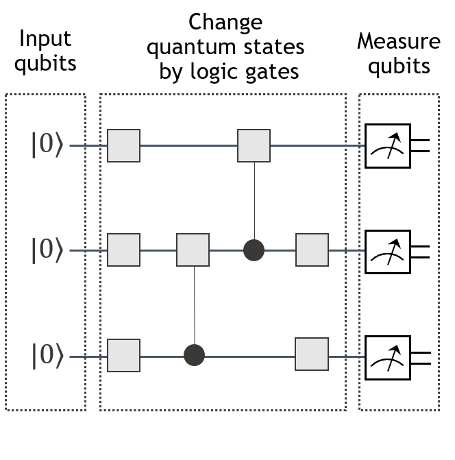
The workflow of quantum computation can be described as a quantum circuit. Each wire corresponds to one qubit, and gates are applied in a left-to-right manner. Some gates have control bits represented by black circles. Gates with control bits are applied only when all the values of control bits match those defined by the users. Measurements are represented by stylized pointer dials, turning a quantum bit (single wire) into a classical bit (double wires). See below for a representative illustration.

Quantum circuit simulation

The task of numerically simulating quantum computation (on a classical computer) is referred to as quantum circuit simulation.

A straightforward quantum circuit simulation can be viewed as a simple matrix-vector multiplication. One takes the unitary matrix corresponding to the gate sequence in a quantum circuit and multiplies it with a column vector representing the input state (usually zero-initialized), and the output state is given by the resulting column vector. The cuStateVec library from the cuQuantum SDK aims to provide a high-performance solution for such a state-vector-based simulation.

However, this naive approach is greatly limited as the problem size scales exponentially in the number of qubits. Moreover, it does not exploit any parallelism, nor is it desired if only partial information is needed (say we only need the expectation value).

To go further beyond the maximum qubit number simulatable on a classical computer (on the order of 50), we need to explore the data sparsity nature of the state vector. The basic idea is while the Hilbert space for state vectors is exponentially large, not all corners of the space are equally important. Following this route, physicists and mathematicians realize that tensor networks are a viable strategy to compress and extract relevant information from an otherwise impossible-to-fully-describe space.

Specifically, a quantum state of N qubits can be thought as a rank-N tensor, which could be broken down into fully contracted, low-rank tensors, potentially turning the complexity of the problem from exponential to polynomial in the qubit number N. Then, the main challenge is transformed to efficiently compute the tensor contractions. The cuTensorNet library from the cuQuantum SDK aims to provide a high-performance solution for tensor network computations.

References

The NVIDIA Technical Blog offers good starting points for learning more about the cuQuantum SDK:

• Accelerating Quantum Circuit Simulation with NVIDIA cuStateVec

• Scaling Quantum Circuit Simulation with NVIDIA cuTensorNet

Citing cuQuantum

• 8. Bayraktar et al., “cuQuantum SDK: A High-Performance Library for Accelerating Quantum Science,” 2023 IEEE International Conference on Quantum Computing and Engineering (QCE), Bellevue, WA, USA, 2023, pp. 1050-1061, doi: 10.1109/QCE57702.2023.00119.