Overview#
This section describes the basic working principles of the cuTensorNet library. For a general introduction to quantum circuits, please refer to Introduction to quantum computing.
Introduction to tensor networks#
Tensor networks emerge in many mathematical and scientific domains, ranging from quantum circuit simulations, quantum many-body physics, and quantum chemistry, to machine learning and probability theory. As network sizes scale up exponentially, there is an ever-increasing need for a high-performance library that can drastically facilitate efficient parallel implementations of tensor network algorithms across multiple domains, which cuTensorNet aims to serve.
Tensor and tensor network#
Tensors are a generalization of scalars (0D), vectors (1D), and matrices (2D), to an arbitrary number of dimensions. In the cuTensorNet library, we follow cuTENSOR’s nomenclature:
A rank (or order) \(N\) tensor has \(N\) modes
Each tensor mode has an extent (the size of the mode) and can be assigned a label (index) as part of the tensor network
Each tensor mode has a stride, reflecting the distance in physical memory between two logically consecutive elements along that mode, in units of elements
For example, a \(3 \times 4\) matrix \(M\) has two modes (i.e., it’s a rank-2 tensor) of extent 3 and 4, respectively. In the C (row-major) memory layout, it has strides (4, 1). We can assign two mode labels, \(i\) and \(j\), to represent it as \(M_{ij}\).
Note
For NumPy/CuPy users, rank/order translates to the array attribute .ndim, the sequence of extents translates to .shape,
and the sequence of strides has the same meaning as .strides but in different units (NumPy/CuPy uses bytes instead of counts).
When two or more tensors are contracted to form another tensor, their shared mode labels are summed over. Diagrammatically, tensors and their contractions can be visualized as follows:
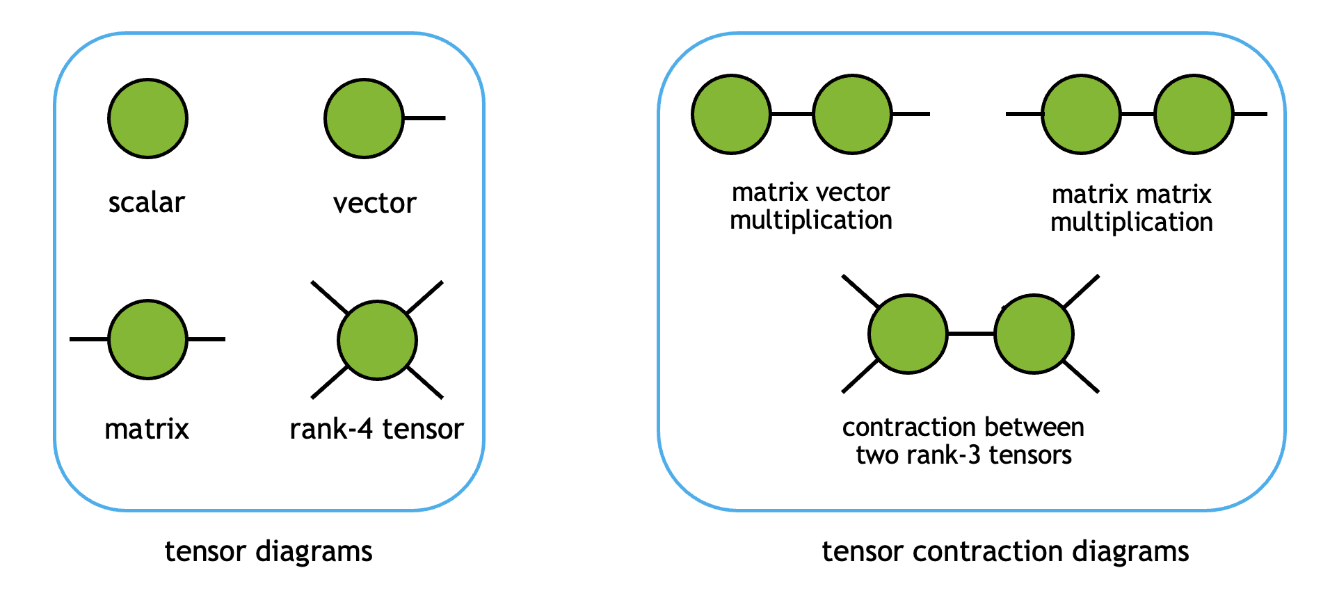
Here, each vertex represents one tensor object, and each edge stands for one tensor mode (label). When a mode label is contracted, the tensors are connected by the corresponding edges.
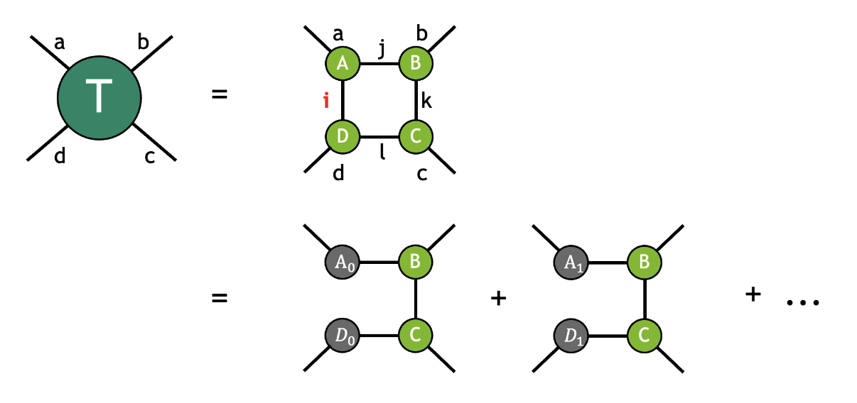
A tensor network is a collection of tensors contracted together to form an output tensor. The contractions between the constituent tensors fully determine the network topology. For example, the tensor \(T\) below is given by contracting the tensors \(A\), \(B\), \(C\), and \(D\):
where the modes with the same label are implicitly summed over following the Einstein summation convention. In this example, the mode label \(i\) connects the tensors \(D\) and \(A\), the mode label \(j\) connects the tensors \(A\) and \(B\), the mode label \(k\) connects the tensors \(B\) and \(C\), the mode label \(l\) connects the tensors \(C\) and \(D\). The four uncontracted modes with labels \(a\), \(b\), \(c\), and \(d\) refer to free modes (sometimes also referred to as external modes), indicating the resulting tensor \(T\) is of rank 4. Following the diagrammatic convention above, this contraction can be visualized as follows:
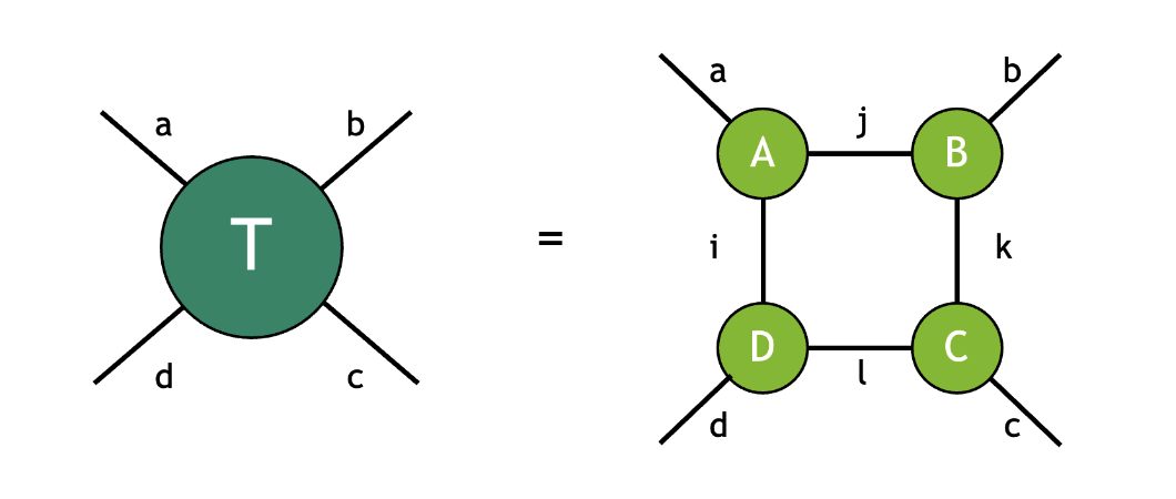
As the diagram shows, this contraction has a square topology with each tensor connected to its adjacent tensors.
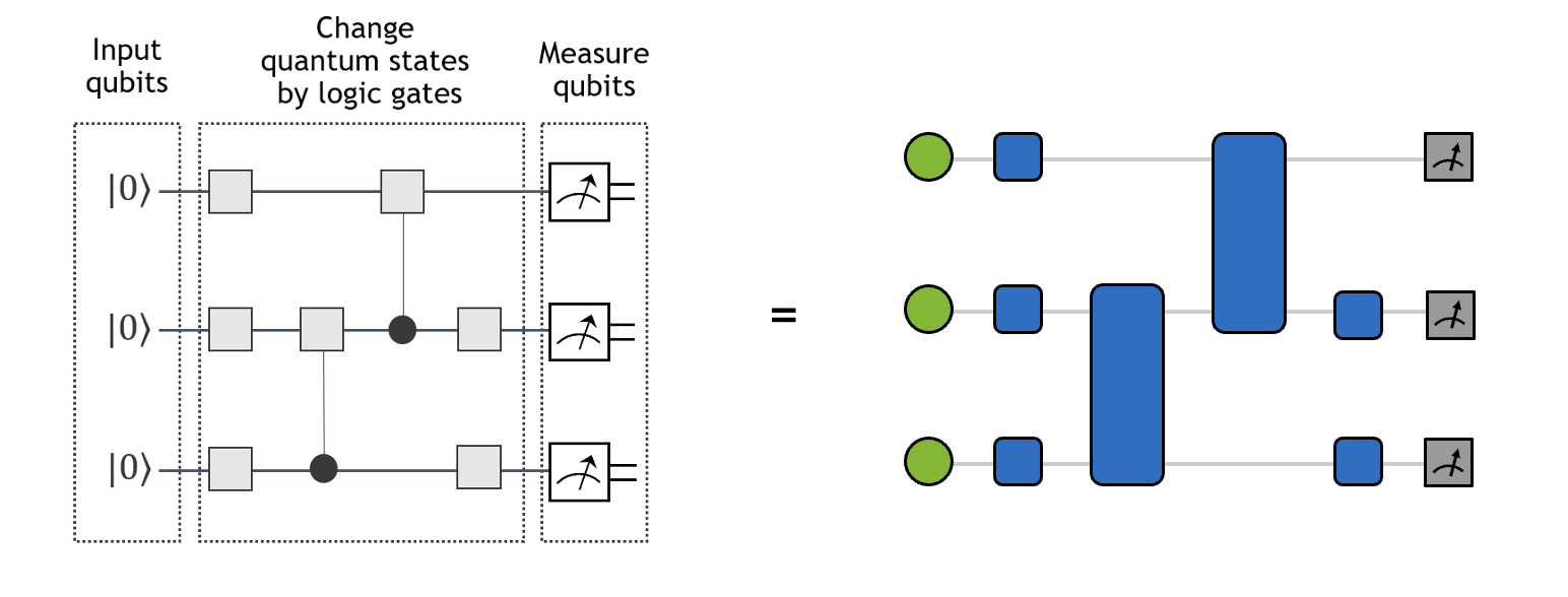
Similarly, a quantum circuit can be viewed as a kind of tensor network. As shown in the figure below, single-qubit and two-qubit gates translate to rank-2 and rank-4 tensors, respectively. Meanwhile, the initial single-qubit states \(|0\rangle\) and single-qubit measurement operations can be viewed as vectors (projectors) of size 2. The contraction of the tensor network on the right yields the wavefunction amplitude of the quantum circuit on the left for a particular basis state (ex: \(|010\rangle\)).
Description of tensor networks#
A full description of a given tensor network contraction requires two pieces of information:
tensor operands and the topology of the tensor network (tensor connectivity hyper-graph).
A tensor network in the cuTensorNet library is represented by the
cutensornetNetworkDescriptor_t descriptor that effectively encodes the topology graph and data
type of the network.
(Network-centric API) To be precise, an empty network gets created via cutensornetCreateNetwork().
Then the modes of each input tensor and the output tensor and their extents are specified by appending a tensor to the
network via cutensornetNetworkAppendTensor() and cutensornetNetworkSetOutputTensor().
The input tensor also accept a qualifiers object in which the tensor can be marked as Conjugate (default non-Conjugate), Constant (default non-Constant), and/or requires Gradient (default false).
Note that there is only one output tensor per tensor network.
When an input tensor is marked as Conjugate, its data will be complex conjugated upon tensor contraction.
When an input tensor is marked as Constant, i.e., its data will not change across subsequent tensor network contractions,
cuTensorNet will invoke a caching mechanism (using the provided CACHE workspace memory)
to accelerate the computation of subsequent tensor network contractions. See Intermediate tensor(s) reuse.
When an input tensor is marked as requires gradient, its corresponding gradient tensor will be computed upon backward propagation call.
After a tensor is appended to the network, its storage (memory buffer and corresponding strides) are specified via cutensornetNetworkSetInputTensorMemory().
The storage for the output tensor are specified via cutensornetNetworkSetOutputTensorMemory().
The storage for input and output tensors need to be provided ahead of contraction or autotuning API calls.
However, it is best if they are provided ahead of contraction preparation call to avoid re-adjusting for different memory alignment or different strides.
Similalry, storage of gradient and adjoint tensors can be provided via cutensornetNetworkSetGradientTensorMemory() and cutensornetNetworkSetAdjointTensorMemory().
The storage for gradient and adjoint tensors need to be provided ahead of gradient computation API call.
However, it is best if they are provided ahead of gradient preparation call to avoid re-adjusting for different memory alignment or different strides.
All network metadata can reside on the host, as constructing a tensor network only requires its topology and data access pattern; we do not need to know the actual content of the input tensors at the tensor network descriptor creation step.
Internally, cuTensorNet utilizes cuTENSOR to create tensor objects and perform pairwise tensor contractions.
cuTensorNet’s APIs are designed such that users can focus on creating the tensor network description without
having to manage such “low-level” details themselves. The tensor network contraction can be computed in different
precisions, specified by the data type given by a cutensornetComputeType_t constant
that can be set to the network via call to cutensornetNetworkSetAttribute() using the constant CUTENSORNET_NETWORK_COMPUTE_TYPE.
If the compute type is not explicitly set, a default compute type is used corresponding to the data type.
Once a valid tensor network is created, one can
Find a cost-optimal tensor network contraction path, possibly with slicing and additional constraints (currently, the cost function can either be the total Flop count or the estimated time to solution)
Access information concerning the tensor network contraction path
Get the needed workspace size to accommodate intermediate tensors
Prepare the tensor network contraction
Auto-tune the network contraction to optimize the run time of the tensor network contraction
Perform the actual tensor network contraction to produce the output tensor, either serially or in parallel
Prepare the tensor network gradients
Compute the gradients of the output tensor with respect to the selected input tensors
It is the user’s responsibility to manage device memory for the workspace (from Step 3) and input/output tensors (for Step 5). See API Reference for the cuTensorNet APIs (section Workspace management API). Alternatively, the user can provide a stream-ordered memory pool to the library to facilitate workspace memory allocations, see Memory management API for details.
Migration guide: plan-based → network-centric API (v2.9.0)#
Starting with cuTensorNet v2.9.0, a network-centric execution flow was introduced to simplify tensor-network definition and execution. The legacy descriptor/plan-based API remains available for backward compatibility but is deprecated. The table below shows a minimal mapping between the two flows:
Plan-based flow (legacy) |
Network-centric flow (preferred) |
|---|---|
create network descriptor: |
create network: cutensornetCreateNetwork |
append inputs via descriptor args ( |
append inputs: cutensornetNetworkAppendTensor |
set output in descriptor ( |
set output: cutensornetNetworkSetOutputTensor |
create optimizer config/info; run cutensornetContractionOptimize |
same; then attach to network if optimizer info object is updated or in distributed settings: cutensornetNetworkSetOptimizerInfo |
compute work sizes: cutensornetWorkspaceComputeContractionSizes and query via cutensornetWorkspaceGetMemorySize |
same |
set workspace: cutensornetWorkspaceSetMemory |
same (SCRATCH/CACHE kinds apply to network flow as well) |
create plan: |
prepare network: cutensornetNetworkPrepareContraction |
autotune: |
network autotune: cutensornetNetworkAutotuneContraction |
run contraction per-slice: |
run contraction: cutensornetNetworkContract (with slice group if desired) |
gradients (experimental legacy): |
gradients (network): set adjoint/gradient buffers via cutensornetNetworkSetAdjointTensorMemory and cutensornetNetworkSetGradientTensorMemory, prepare via cutensornetNetworkPrepareGradientsBackward, compute via cutensornetNetworkComputeGradientsBackward |
Key behavioral notes:
Input/output memory is attached in the network flow using cutensornetNetworkSetInputTensorMemory and cutensornetNetworkSetOutputTensorMemory.
CACHE workspace is required to compute gradients (stores intermediates for backward propagation). Use cutensornetWorkspaceSetMemory with
CUTENSORNET_WORKSPACE_CACHE.To preserve previous semantics for repeated runs with constant inputs, mark constants via qualifiers when appending tensors, and keep CACHE workspace configured.
Tensor network state specification and processing#
To simplify the specification and processing of tensor networks (TN) encountered in quantum science and other domains, cuTensorNet provides a set of TN state API functions for users to gradually build a given tensor network state and subsequently compute its properties:
cutensornetCreateState()is used to create the initial (vacuum) tensor network state in some direct-product tensor space specified by dimensions of all of its constituent vector spaces, such as qudit spaces or, more commonly, qubit spaces (all vector space dimensions are equal to 2 for qubits).Apply the required tensor operators to gradually build the tensor network of interest (e.g., a given quantum circuit):
cutensornetStateApplyTensorOperator()(cutensornetStateApplyTensor()deprecated) is used to apply general tensor operators (e.g., quantum gates) to a tensor network state, defining the final tensor network state in the direct-product tensor space.
cutensornetStateApplyDiagonalTensorOperator()is used to apply a diagonal tensor operator to the tensor network state. A diagonal tensor operator is a tensor in which all off-diagonal elements are zero, acting multiplicatively only on the diagonal entries of the state modes it covers. For \(n\) state modes, it is fully characterized by a rank-\(n\) tensor containing the diagonal values (e.g., for a 2-qubit diagonal gate like CZ, only 4 diagonal elements are needed instead of a full \(4 \times 4\) matrix). This provides a more memory-efficient representation for diagonal quantum gates.
cutensornetStateApplyControlledTensorOperator()is used to apply a controlled tensor operator to the tensor network state. This API uses the control-target representation typical for multi-qubit quantum gates. This is useful for gates like CNOT, Toffoli, and other controlled unitaries.
cutensornetStateApplyNetworkOperator()is used to apply a tensor network operator (defined viacutensornetNetworkOperator_t) to the tensor network state. This allows applying complex operators such as matrix product operators (MPOs) to the state.
cutensornetStateApplyUnitaryChannel()andcutensornetStateApplyGeneralChannel()are used to apply quantum channels to the tensor network state. Unitary channels are defined by a set of unitary Kraus operators with associated probabilities, while general channels support non-unitary Kraus operators for modeling noise and decoherence.Once the tensor network state of interest (e.g., the output state of a quantum circuit) has been constructed, its properties can be computed:
cutensornetCreateAccessor()specifies a slice of a tensor network state that needs to be computed, to inspect the amplitudes of the tensor network state without producing the full state tensor.
cutensornetCreateExpectation()specifies the expectation value of a given tensor network operator over a given tensor network state. Currently, supported tensor network operators include those defined as a sum of products of tensors acting on disjoint subsets of tensor network state modes, as well as a sum of matrix product operators. In particular, the Jordan-Wigner transformation produces a subclass of the first category. SeecutensornetNetworkOperator_tfor more information.
cutensornetCreateMarginal()specifies a marginal distribution tensor to be computed for a given tensor network state. In physics literature, a marginal distribution tensor is referred to as the Reduced Density Matrix (RDM). It is the tensor obtained by tracing the direct product of the defined tensor network state with its conjugate state (from the dual direct-product tensor space) over the specified tensor modes.
cutensornetCreateSampler()creates a tensor network state sampler that can sample the tensor network state over specified (either all or a subset of the) tensor modes. When sampling over all tensor state modes, the tensor network state defines the probability distribution in the corresponding direct-product tensor space. Namely, the squared absolute value of each tensor element defines its probability of appearing as a sample in the sampling procedure. In quantum circuit simulations, this would mean generating the output samples from the final state of the quantum circuit according to their probabilities. Sampling over an incomplete set of tensor network state modes would refer to sampling the corresponding marginal probability distribution.
Expectation value gradients#
For variational optimization and automatic differentiation-style workflows, cuTensorNet can evaluate the expectation value \(E = \langle\psi|H|\psi\rangle\) and, in the same execution, write gradients \(\partial E / \partial A_j\) for tensor operators \(A_j\) that were registered when the state was built.
The typical flow is:
Apply each operator that should receive a gradient with cutensornetStateApplyTensorOperatorWithGradient(), passing a pre-allocated device buffer (and optional strides) with the same shape as the operator data; gradients are written to these buffers when the backward pass runs. The target buffer may be changed later via cutensornetStateUpdateTensorOperatorGradient(). Registrations must be in place before cutensornetExpectationPrepare() so that workspace sizing accounts for gradient computation.
Create the expectation with cutensornetCreateExpectation(). Then prepare with cutensornetExpectationPrepare() as for a standard expectation evaluation. SCRATCH workspace must be configured (query the required size after prepare).
Call cutensornetExpectationComputeWithGradientsBackward(). Supply
expectationValueAdjointas a host scalar upstream gradient for the chain rule; set it to \(1\) to obtain \(\partial E/\partial A_j\) directly. Use theaccumulateGradientsflag to add into existing gradient buffers instead of overwriting them.
A commented C sample is provided under Code example (expectation value with gradients).
Approximate tensor network algorithms#
While tensor network contraction path optimization can greatly reduce the computational cost of the exact contraction of a tensor network, the cost can still quickly scale beyond the classical computer’s limit as the network size and complexity increase. A variety of approximate tensor network methods have been developed to address this challenge, such as algorithms based on the matrix product states (MPS). These methods often aim to exploit the sparsity in the tensor network, using tensor decomposition techniques such as QR and SVD.
The QR and SVD decompositions of a tensor can be visualized by the diagram below and can be viewed as the higher-order generalization of matrix QR/SVD.
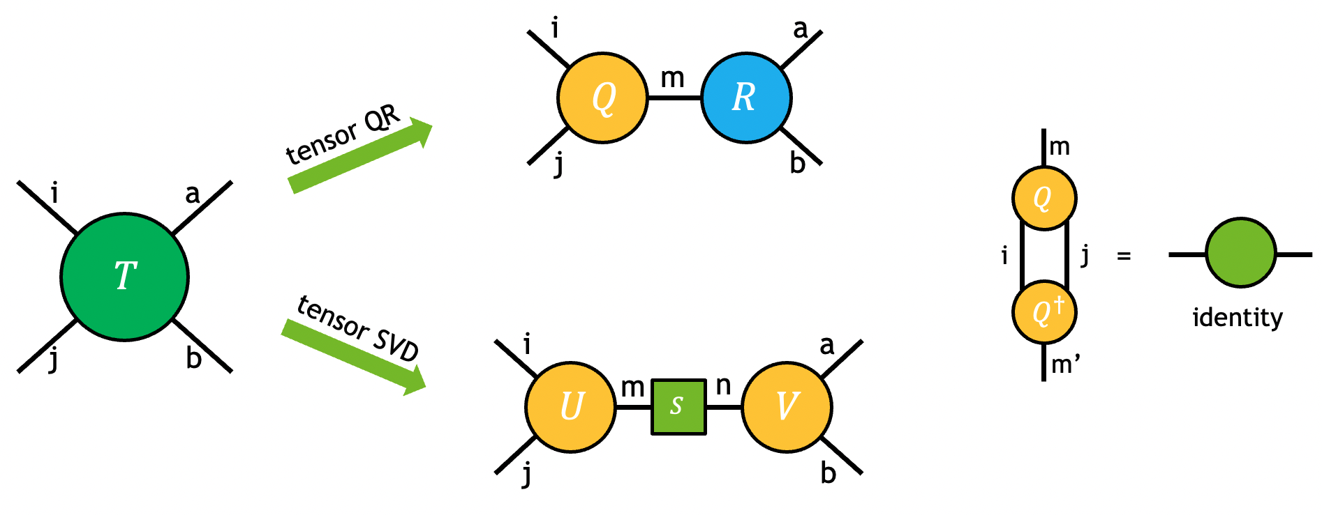
The problem can be fully specified by user-requested partitions of modes in the output tensors. For example, the tensor \(T\) in the figure above is decomposed into output tensors \(U\), \(S\), and \(V\) using tensor SVD:
Note
Although the output \(S\) is represented as a matrix in the equation and the diagram, only its diagonal elements are nonzero. In all SVD-related APIs of cuTensorNet, only the non-zero diagonal elements are returned (as a vector).
Once the partition of modes in \(U\) and \(V\) is determined, input tensor \(T\) is first permuted to an intermediate tensor \(\bar{T}\) with the proper mode ordering such that it can be viewed as a matrix for the decomposition:
After the matrix SVD/QR decomposition, permutation may still be needed to transform the output intermediate tensors \(\bar{U}\) and \(\bar{V}\), to the requested output \(U\) and \(V\).
Note
Tensor SVD and QR in cuTensorNet operate in reduced mode, i.e., \(k=min(m, n)\) where k denotes the extent of the shared mode of the output, while m and n represent the effective input matrix row/column sizes. While tensor QR is always exact, cuTensorNet provides different ways for users to truncate singular values, \(\bar{U}\), and \(\bar{V}\). For instance, if the user wishes to perform fixed extent truncation in tensor SVD, \(k\) can be set to be lower than \(min(m, n)\). See SVD options for detailed descriptions.
In practice, tensor decomposition and pairwise tensor contraction are often combined to transform the original network to a new topology that reflects its internal sparsity or entanglement geometry in the field of quantum simulation. For instance, in the matrix product states (MPS) simulator, the qubits states are mapped to a 1-dimensional tensor chain. When gate tensors are applied to the MPS, a sequence of contraction and tensor QR/SVD operations are performed to ensure that the output states are still represented as a 1-dimensional tensor chain. The compound operation that is used to maintain the MPS geometry is termed as the gate split process. For example, a two-qubit gate tensor \(G\) is applied to two connecting tensors \(A\) and \(B\) to generate output tensors \(\tilde{A}\) and \(\tilde{B}\) with similar modes as \(A\) and \(B\):
In the gate split process, the number of singular values may also be truncated to keep the MPS size tractable. By iterating this process throughout the network, the original tensor network can be approximated by the output MPS states. The process can be diagrammatically shown as below:
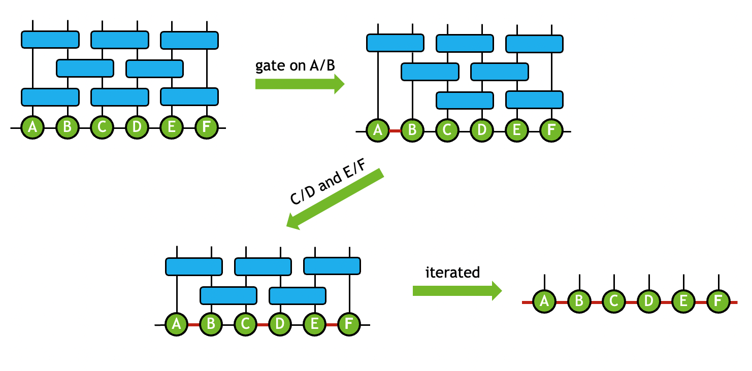
For more detailed explanation of how the transformation is performed, please refer to Gate Split Algorithm below.
Projection Matrix Product State#
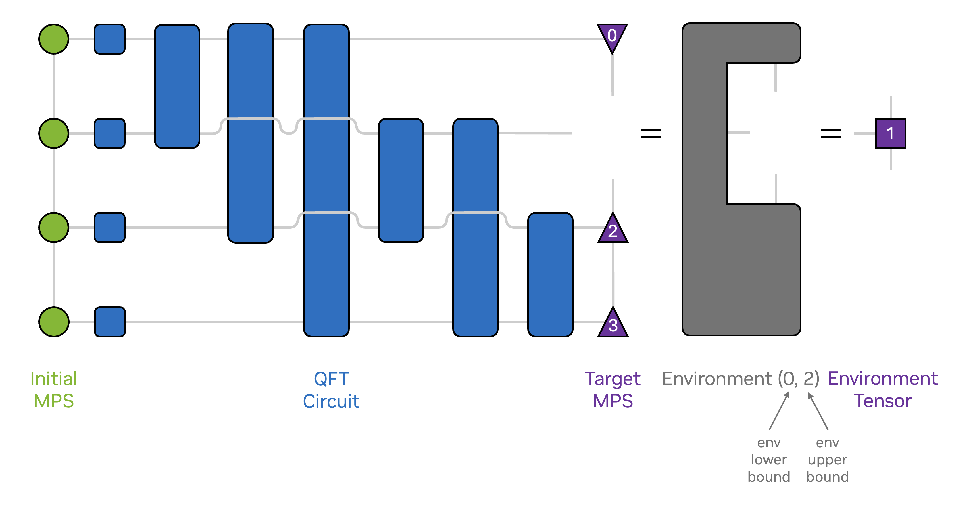
An alternative approach to approximately simulate a quantum circuit is to variationally optimize the tensors in an iterative, sweeping fashion. The so-called circuit density matrix renormalization group (circuit DMRG) algorithm is a popular example of this approach and works well for circuits that can be split into horizontal components. Circuit DMRG and other variational methods rely on projecting the quantum state (or its variation) to be approximated into a compact basis defined by the majority of the tensors of the current MPS approximation of the quantum state. The only tensors which are not included in constructing this basis are the tensors to be variationally optimized in the current iteration.
The following figure illustrates the tensor network corresponding to such a projection.
We offer the projection MPS API to support such projection-based methods:
cutensornetCreateStateProjectionMPS()is used to create the initial projection MPS instance,cutensornetStateProjectionMPS_t.The arguments
numStates,tensorNetworkStates[], andcoeffs[]specify the linear superposition of quantum states (each composed of a set of tensor operators and an initial state, which defaults to the vacuum).As of cuTensorNet v2.9.0, only a single initial state is supported.
The initial MPS approximation to the linear superposition of quantum states is specified by the user-provided buffers passed as the
dualTensors[]argument, which will be modified in-place by several other APIs introduced in the following. In the following we will refer to the current MPS approximation as “dual state” or “target state”. Note that the MPS tensors’ adjoint enters into the environment tensor network depicted in the figure above, but the provided MPS tensors themselves are supplied and written to in their non-conjugated form.Note that the extents of these initially provided buffers constitute an upper bound to the extents of the MPS tensors used over the lifetime of the projection MPS instance. Furthermore, the extents of the MPS tensors are required to not be overcomplete, i.e. the dimension of the mode connecting two MPS tensors cannot exceed the product of qudit dimensions to the left and to the right of said mode in the MPS.
Currently, the extents of the MPS tensors are constant over the lifetime of the projection MPS instance, but additional functionality is planned which will allow for dynamic extents.
The
symmetricargument specifies whether the initial state of all tensor network states is replaced by the target state MPS when contracting environment networks via thecutensornetStateProjectionMPSComputeTensorEnv()API.Algorithms such as circuit DMRG require distinct initial and target states (
symmetric=0) while other variational methods such as the time-dependent variational principle (TDVP) or conventional DMRG for finding extremal eigenvalues of a quantum operator, require the initial and target states to be the same (symmetric=1).The tensors which are to be optimized over the lifetime of the
cutensornetStateProjectionMPS_tinstance are specified by theenvSpecsargument, which is an array ofcutensornetStateProjectionMPSEnvSpec_t.cutensornetStateProjectionMPSEnvSpec_tis a pair of integers, the qudit indices to the left and to the right of the set of MPS tensors to be optimized. Currently only single-site environments are supported, i.e. the distance between lower and upper bound is required to be two. SincecutensornetStateProjectionMPSEnvSpec_tis used to specify both the environment network and a component of the MPS approximation, we will differentiate between the two by using the terms environment and region respectively.
cutensornetStateProjectionMPSComputeTensorEnv()computes the environment tensor for a given environment, as shown in the figure above for the case of acutensornetStateProjectionMPS_tconstructed with argumentsymmetric=0.cutensornetStateProjectionMPSExtractTensor()extracts the tensor for a region of the MPS of the target state in its unconjugated form.Note that for the currently exposed functionality, this API performs orthogonalization of the MPS tensors towards the region
envSpec, and thus may modify all MPS tensors in the target state.
cutensornetStateProjectionMPSInsertTensor()inserts a tensor into a region of the MPS of the target state, overwriting the current values of the target state MPS tensors.For the currently exposed functionality, this API only modifies the MPS tensors within the region.
cutensornetStateProjectionMPSUpdateDualTensors()updates the dual MPS tensor buffers used by the MPS projection.This function allows updating the data pointers for all dual MPS tensors after the projection MPS instance has been created.
The extents and strides of the updated tensors must match those specified at instance creation.
cutensornetStateProjectionMPSUpdateCoefficients()updates the scalar coefficients of the linear superposition of tensor network states.This function may be called multiple times to change the coefficients over the lifetime of the projection object.
The extract-compute-insert cycle#
The cutensornetStateProjectionMPSExtractTensor(), cutensornetStateProjectionMPSComputeTensorEnv(), and cutensornetStateProjectionMPSInsertTensor() APIs form a compute cycle with the following constraints:
cutensornetStateProjectionMPSExtractTensor()initiates a compute cycle. It extracts the tensor for a region and performs orthogonalization of the MPS tensors towards that region.
cutensornetStateProjectionMPSComputeTensorEnv()may optionally be called during a compute cycle to compute the environment tensor.
cutensornetStateProjectionMPSInsertTensor()concludes a compute cycle. It must be called after extraction before another extraction can be performed.
cutensornetStateProjectionMPSUpdateDualTensors()cannot be called during a compute cycle (i.e., between extraction and insertion).
We refer to the Projection MPS Circuit DMRG Example for a complete example of the workflow.
Contraction optimizer#
A contraction path is a sequence of pairwise contractions represented in the numpy.einsum_path() format.
For a given tensor network, the contraction cost can differ by orders of magnitude, depending on the quality of the contraction path.
Therefore, it is crucial to use a path optimizer to find a contraction path that minimizes the total cost of contracting the tensor network.
Currently, the contraction cost can refer to the total floating point operations (FLOP) or the estimated time to solution for the cuTensorNet path optimizer’s purpose, and an optimal
contraction path corresponds to the path with the minimal contraction cost.
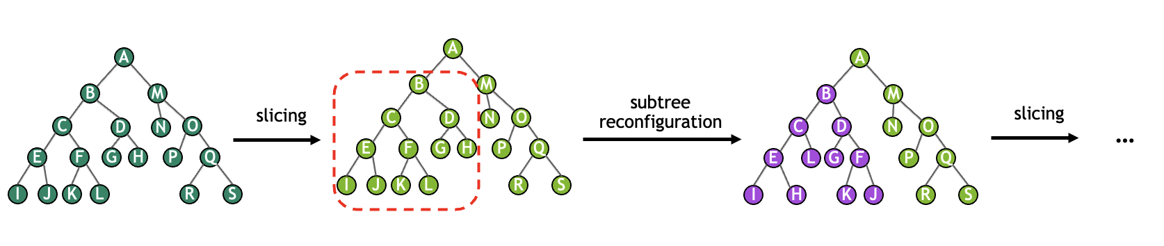
The cuTensorNet path optimizer is based on a graph-partitioning approach (called phase 1), followed by interleaved slicing and reconfiguration optimization (called phase 2).
Practically, experience indicates that finding an optimal contraction path can be sensitive to the choice of configuration parameters,
which can be configured via cutensornetContractionOptimizerConfigSetAttribute() and queried via cutensornetContractionOptimizerConfigGetAttribute(). The rest of this section aims to introduce the overall optimization scheme and these configurable parameters.
Once the optimization completes, it returns an opaque object cutensornetContractionOptimizerInfo_t that contains all of the attributes for creating a contraction plan. For example, the optimal path (CUTENSORNET_CONTRACTION_OPTIMIZER_INFO_PATH) and the corresponding FLOP count (CUTENSORNET_CONTRACTION_OPTIMIZER_INFO_FLOP_COUNT) can be queried via cutensornetContractionOptimizerInfoGetAttribute().
Note
The returned FLOP count assumes the input tensors are real-valued; for complex-valued tensors, multiplying it by 4 is a good estimation.
Alternatively, we can bypass the cuTensorNet optimizer entirely by supplying your own path using cutensornetContractionOptimizerInfoSetAttribute(). For the unset cutensornetContractionOptimizerInfo_t attributes (ex: the number of slices and the FLOP) cuTensorNet will either use the default values or compute them on the fly when applicable.
Graph partitioning#
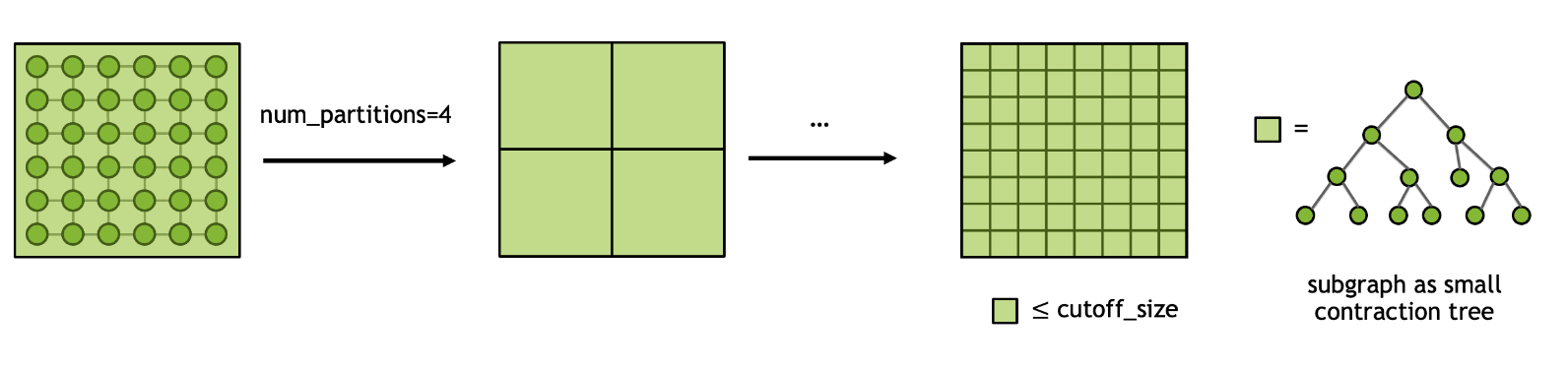
In general, searching for the optimal contraction path for a given tensor network is a NP-hard problem. Therefore, it is crucial to approach this problem in a divide-and-conquer spirit. Given an input tensor network, we first perform graph partitioning to split the network into N smaller subgraphs and repeat this process recursively until the size of each subgraph is less than the cutoff size. Once the final partitioning scheme is determined, finding the paths for contracting first within each subgraph and then all subgraphs become tractable. The process can be illustrated using the diagram below and we get a coarse contraction path or contraction tree for subsequent optimizations.
The cuTensorNet library provides controls over the graph partition algorithms through the following parameters:
CUTENSORNET_CONTRACTION_OPTIMIZER_CONFIG_GRAPH_NUM_PARTITIONS: The number of subgraphs to partition into within each loop.
CUTENSORNET_CONTRACTION_OPTIMIZER_CONFIG_GRAPH_CUTOFF_SIZE: The maximal size allowed for each subgraph until the partitioning is completed.
CUTENSORNET_CONTRACTION_OPTIMIZER_CONFIG_GRAPH_ALGORITHM: The graph algorithm to be used in graph partitioning. The default is set to CUTENSORNET_GRAPH_ALGO_KWAY.
CUTENSORNET_CONTRACTION_OPTIMIZER_CONFIG_GRAPH_IMBALANCE_FACTOR: The maximum allowed size imbalance among the partitions.
CUTENSORNET_CONTRACTION_OPTIMIZER_CONFIG_GRAPH_NUM_ITERATIONS: The number of iterations for the refinement algorithms at each stage of the uncoarsening process of the graph partitioner.
CUTENSORNET_CONTRACTION_OPTIMIZER_CONFIG_GRAPH_NUM_CUTS: The number of different partitionings that the graph partitioner will compute.
Slicing#
In order to fit a tensor network contraction into available device memory, as specified by workspaceSizeConstraint, it may be necessary to use slicing (also known as variable projection or bond cutting).
By slicing, we split the contraction of the entire tensor network into a number of independent smaller contractions where each contraction considers only one particular position
of a certain mode (or combination of modes). The total number of slices that are created equals the product of the extents of the sliced modes.
The result for full tensor network contraction can be obtained by summing over the output of each sliced contraction.
Taking the above \(T\) tensor as an example, if we slice over the mode i we obtain the following representation:
As one can see from the diagram, the sliced mode \(i_s\) is no longer implicitly summed over as part of tensor contraction, but instead explicitly summed in the last step. As a result, slicing can effectively reduce the memory footprint for contracting large tensor networks, in particular quantum circuits. Besides, since each sliced contraction is independent from the others, the computation can be efficiently parallelized in various distributed settings.
Despite all the benefits above, the downside of slicing is that it often increases the total FLOP count of the entire contraction. The overhead of slicing heavily depends on the contraction path and the modes that are sliced. In general, there is no simple way to determine the best set of modes to slice.
The slice-finding algorithm in the cuTensorNet library can be tuned by the following parameters:
CUTENSORNET_CONTRACTION_OPTIMIZER_CONFIG_SLICER_DISABLE_SLICING: If set to 1, slicing will not be considered, regardless of available memory. The default is 0.
CUTENSORNET_CONTRACTION_OPTIMIZER_CONFIG_SLICER_MEMORY_MODEL: Specifies the memory model used to determine the workspace size, seecutensornetMemoryModel_t. The default is to use a memory model compatible with cuTENSOR (CUTENSORNET_MEMORY_MODEL_HEURISTIC).
CUTENSORNET_CONTRACTION_OPTIMIZER_CONFIG_SLICER_MEMORY_FACTOR: The memory limit for the first slice-finding iteration as a percentage of the workspace size. The default is 80 when usingCUTENSORNET_MEMORY_MODEL_CUTENSORfor the memory model and 100 when usingCUTENSORNET_MEMORY_MODEL_HEURISTIC.
CUTENSORNET_CONTRACTION_OPTIMIZER_CONFIG_SLICER_MIN_SLICES: Specifies the minimum number of slices to produce (e.g. to create parallelizable work). The default is 1.
CUTENSORNET_CONTRACTION_OPTIMIZER_CONFIG_SLICER_SLICE_FACTOR: Specifies the factor by which the number of slices will increase per slice-finding iteration. For example, if the previous iteration had \(N\) slices and the slice factor is \(s\), the next iteration will produce at least \(sN\) slices. Since reconfiguration (see below) occurs after each slice-finding iteration, increasing this value will decrease the amount of reconfiguration, which, in turn, will decrease the amount of time taken but probably worsen the quality of the contraction tree. The default is 32. Must be at least 2. A small value of this factor (for example 2 or 4) is recommended when the number of slices requested or required is very large, because it provides a better quality of slices.
The slice-finding algorithm in the cuTensorNet library utilizes a set of heuristics and the process can be coupled with the subtree reconfiguration routine to
find the optimal set of modes that both satisfies the memory constraint and incurs the least overhead.
Reconfiguration#
At the end of each slice-finding iteration, the quality of the contraction tree has been diminished by the slicing. We can improve the contraction tree at this stage by performing reconfiguration. Reconfiguration considers a number of small subtrees within the full contraction tree and attempts to improve their quality. The repeated process of slicing and reconfiguration can be viewed as illustrated in the diagram below.
Although this process is computationally expensive, a sliced contraction tree without reconfiguration may be orders of magnitude more expensive to execute than expected. The cuTensorNet library offers some controls to influence the reconfiguration algorithm:
CUTENSORNET_CONTRACTION_OPTIMIZER_CONFIG_RECONFIG_NUM_ITERATIONS: Specifies the number of subtrees to consider during each reconfiguration. The amount of time spent in reconfiguration, which usually dominates the optimizer run time, is linearly proportional to this value. Based on our experiments, values between 500 and 1000 provide very good results. The default is 500. Setting this to 0 will disable reconfiguration.
CUTENSORNET_CONTRACTION_OPTIMIZER_CONFIG_RECONFIG_NUM_LEAVES: Specifies the maximum number of leaf nodes in each subtree considered by reconfiguration. Since the time spent is exponential in this quantity for optimal subtree reconfiguration, selecting large values will invoke faster non-optimal algorithms. Nonetheless, the time spent by reconfiguration increases very rapidly as this quantity is increased. The default is 8. Must be at least 2. While using the default value usually produces the best FLOP count, setting it to 6 will speed up the optimizer execution without a significant increase in the FLOP count for many problems.
Deferred rank simplification#
Since the time taken by the path-finding algorithm increases quickly as the number of tensors increases, it is advantageous to minimize the number of tensors, if possible. Rank simplification removes trivial tensor contractions from the network in order to improve performance. These contractions are those where a tensor is only connected with at most two neighbors, effectively making the contraction a small matrix-vector or matrix-matrix multiplication. One example for rank simplification is given in the figure below:
This technique is particularly useful for tensor networks with low connectivity; for instance, all single-qubit gates in quantum circuits can be fused with the neighboring multi-qubit gates, thereby reducing the search space for the optimizer. The necessary contractions to perform the simplification are not performed immediately but are instead prepended to the returned contraction path. If, for some reason, such simplification is not desired, it can be disabled:
CUTENSORNET_CONTRACTION_OPTIMIZER_CONFIG_SIMPLIFICATION_DISABLE_DR: If set to 1, simplification will be skipped. This will run the path-finding algorithm on the full tensor network, increasing the time needed. The default is 0.
While simplification helps lower the FLOP count in most cases, it may sometimes (depending on the network topology and other factors) lead to a path with a higher FLOP count. We recommend that users experiment with the impact of turning simplification off (using the option listed above) on the computed path.
Hyper-optimizer#
cuTensorNet provides a hyper-optimizer for the path optimization that can automatically generate
many instances of contraction paths and return the best of them in terms of the total FLOP count.
The number of instances is user-controlled via the use of CUTENSORNET_CONTRACTION_OPTIMIZER_CONFIG_HYPER_NUM_SAMPLES which is set to 0 by default.
The idea here is that the hyper-optimizer will create
CUTENSORNET_CONTRACTION_OPTIMIZER_CONFIG_HYPER_NUM_SAMPLES instances, each reflecting the use of different parameters within the optimizer algorithm.
Each instance will run the full optimizer algorithm including reconfiguration and slicing (if requested).
At the end of the hyper-optimizer loop, the best path (in term of FLOP counts) is returned.
The hyper-optimizer runs its instances in parallel.
The desired number of threads can be set using CUTENSORNET_CONTRACTION_OPTIMIZER_CONFIG_HYPER_NUM_THREADS
and is chosen to be half of the available logical cores by default. The number of threads
is limited to the number of the available logical cores to avoid the resource contention that is likely with a larger number of threads.
Internally, cuTensorNet holds a thread pool for multithreading in the hyper-optimizer, etc. The thread pool lifetime is bound to the cuTensorNet handle. (In previous releases, OpenMP was used; this is no longer the case since cuTensorNet v2.0.0.)
The configuration parameters that are varied by the hyper-optimizer can be found in the graph partitioning section.
Some of these parameters may be fixed to a given value (via cutensornetContractionOptimizerConfigSetAttribute()). When a parameter is fixed, the hyper-optimizer will not randomize it. The randomness can be fixed by setting the seed via the attribute CUTENSORNET_CONTRACTION_OPTIMIZER_CONFIG_SEED.
Intermediate tensor(s) reuse#
cuTensorNet currently supports caching/reuse of intermediate tensors for cases where some of the input tensors vary in value, but the network structure does not. In such cases, it can drastically accelerate repeated executions of the same tensor network where some tensors update their values. One example is calculation of the probability amplitudes of individual bit-strings or small batches of them, the procedure often used for the verification/validation of quantum processors. In this case, only the calculation of the first bit-string amplitude incurs the full computational cost whereas the subsequent calculations of bit-string probability amplitudes should run much faster, benefiting from the intermediate tensor caching/reuse. Another example is the sampling of the probability distribution of the final quantum circuit state. The sampling procedure will also benefit from intermediate reuse since the underlying reduced density matrices computed for groups of qubits do not change their structure while only updating the values of a relatively small number of input tensors. Finally, variational quantum algorithms with a relatively small number of variational parameters may also be accelerated with this new feature.
To activate intermediate tensor reuse for constant input tensors, users need to:
Mark the constant input tensors when constructing the network (
cutensornetCreateNetworkDescriptor()) using thecutensornetTensorQualifiers_tparameter, by setting theisConstanttag on each constant input tensor.Provide cache workspace to store the intermediate tensors (use
cutensornetWorkspaceSetMemory()withCUTENSORNET_WORKSPACE_CACHEworkspaceKind parameter). When both these inputs are provided, cuTensorNet will utilize the cache workspace to accelerate repeated contractions of the same tensor network.
Approximation setting#
SVD Options#
In addition to the standard tensor SVD mentioned above, cuTensorNet allows users to perform truncation, normalization, and re-partition
during the decomposition using various SVD algorithms. For truncation, the most common strategy is to keep the largest k number of singular values and trim out the remaining ones.
In cuTensorNet, this can be easily specified by modifying the extent of the shared mode in the output cutensornetTensorDescriptor_t object.
Alternatively, users may truncate the singular values based on the actual value or the distribution of the eigenvalues during runtime.
Such truncation setting, SVD algorithm along with normalization and re-partition options are provided by different attributes of the cutensornetTensorSVDConfig_t object:
CUTENSORNET_TENSOR_SVD_CONFIG_ABS_CUTOFF: The cutoff for the largest singular value during truncation. Eigenvalues that are smaller will be trimmed out.
CUTENSORNET_TENSOR_SVD_CONFIG_REL_CUTOFF: The cutoff for the maximal singular value relative to the largest eigenvalue. Eigenvalues that are smaller than this fraction of the largest singular value will be trimmed out.
CUTENSORNET_TENSOR_SVD_CONFIG_S_NORMALIZATION: Whether to normalize certain norm of the truncated singular values to 1. The default is no.
CUTENSORNET_TENSOR_SVD_CONFIG_S_PARTITION: Whether to partition the singular values onto u, or v, or both u and v. The default is no.
CUTENSORNET_TENSOR_SVD_CONFIG_ALGO: Which SVD algorithm to use. The default isGESVD.
CUTENSORNET_TENSOR_SVD_CONFIG_ALGO_PARAMS: Optional, the custom parameters for certain SVD algorithms (currently supports GESVDJ and GESVDR). For the default setting corresponding to GESVDJ and GESVDR, please refer tocutensornetGesvdjParams_tandcutensornetGesvdrParams_t, respectively.
CUTENSORNET_TENSOR_SVD_CONFIG_DISCARDED_WEIGHT_CUTOFF: The cutoff for the cumulative discarded weight (square sum of discarded singular values divided by square sum of all singular values). Eigenvalues with cumulative discarded weight will be trimmed out.
Note
The value-based truncation options in cutensornetTensorSVDConfig_t can be used in conjunction with the fixed extent truncation, but since the actual reduced extent found at runtime is unknown,
the size of the data allocation for the output tensors should always be based on the assumption of no value-based truncation. After the execution, the potentially reduced extent found at runtime will
be stored in the CUTENSORNET_TENSOR_SVD_INFO_REDUCED_EXTENT attribute of cutensornetTensorSVDInfo_t and also reflected in the output cutensornetTensorDescriptor_t.
Users can either call cutensornetTensorSVDInfoGetAttribute() or cutensornetGetTensorDetails() to query this information.
Gate-split algorithm#
In general, there is more than one approach to perform the gate split operation.
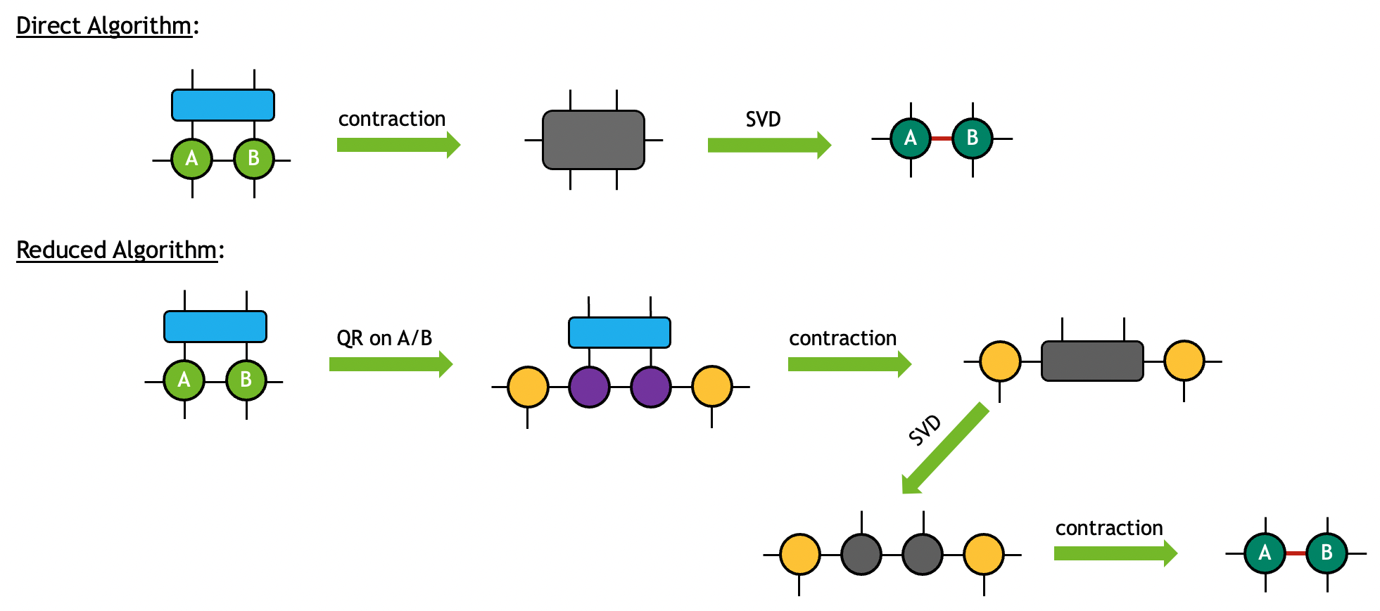
cuTensorNet provides two algorithms in cutensornetGateSplitAlgo_t for this purpose:
CUTENSORNET_GATE_SPLIT_ALGO_DIRECT: The three input tensors will first be contracted to form an intermediate tensor. A subsequent tensor SVD will take place to decompose the intermediate tensor to the desired output. This algorithm is generally more memory-demanding but more performant when the tensor sizes are relatively small.
CUTENSORNET_GATE_SPLIT_ALGO_REDUCED: The input tensors A and B will first be decomposed into smaller fragments via tensor QR. The twoRtensors from the decomposition will then be contracted with input tensorGto form an intermediate tensor. A subsequent tensor SVD will take place to decompose the intermediate tensor, the output of which will then contract with theQtensors from the first step to form the desired outputs. This algorithm is generally less memory demanding and more performant when the tensors sizes get large.
Note
For CUTENSORNET_GATE_SPLIT_ALGO_REDUCED, cuTensorNet may internally skip QR on tensor A or/and B if no memory size reduction
can be achieved in the decomposition.
The two algorithms can be diagrammatically visualized as follows (singular values are partitioned equally onto the two outputs in this example):
Supported data types#
For tensor network contraction, a valid combination of the data and compute types is inherited in a straightforward fashion from
that of cuTENSOR. Please refer to cutensornetCreateNetworkDescriptor() and cuTENSOR’s User Guide for details.
For approximate tensor network functionalities including tensor SVD/QR decompositions and gate split operation, the following data types are supported:
Note
For gate split operation, the valid compute types for the data types above are consistent with that of tensor network contraction.
References#
For a technical introduction to cuTensorNet, please refer to the NVIDIA blog:
For further information about general tensor networks, please refer to the following:
For the application of tensor networks to quantum circuit simulations, please see:
Citing cuQuantum#
Bayraktar et al., “cuQuantum SDK: A High-Performance Library for Accelerating Quantum Science,” 2023 IEEE International Conference on Quantum Computing and Engineering (QCE), Bellevue, WA, USA, 2023, pp. 1050-1061, doi: 10.1109/QCE57702.2023.00119.